Lesson 6: Eigenvectors and Eigenvalues

Goal

Understand the special directions in which a linear map acts like scalar multiplication, and learn how to recognize them from the equation $Av = λv$ .

By the end of the lesson, you should be able to say, in plain language, what an eigenvector is, what an eigenvalue is, and why the determinant condition $det(A - λI) = 0$ appears.

Motivation

Most vectors change direction when a matrix acts on them.

That is the ordinary case.

The interesting case is when a matrix has a direction it does not twist at all. It may stretch that direction, shrink it, or flip it, but it does not send it somewhere else.

That is the feature behind eigenvectors.

The idea matters because repeated application of a matrix becomes easy along those directions. It also matters because covariance matrices, stability analyses, and dimensionality-reduction methods all lean on the same geometry.

Prerequisites

Lesson 1: Vectors.
Lesson 2: Matrices as Linear Transformations.
Lesson 3: Matrix Multiplication.
Lesson 4: Determinants.
Lesson 5: Inverse Matrices.
The meaning of scalar multiplication and matrix-vector multiplication.

Notation / Symbol Table

Symbol	Plain-English name	Meaning
$A$	matrix	A square matrix or linear transformation acting on vectors.
$v$	vector	A candidate eigenvector; it must be nonzero.
$\lambda$	eigenvalue	The scalar factor by which $A$ stretches or flips $v$ .
$I$	identity matrix	The matrix that leaves vectors unchanged.
$Av = λv$	eigenvector equation	The defining relationship for an eigenpair.
$\det(A - λI)$	characteristic determinant	The polynomial condition used to find eigenvalues.

Core Ideas

The invariant-direction idea

If a matrix sends a vector back onto the same line, that vector is special.

Formally, a nonzero vector $v$ is an eigenvector of $A$ if

Av = λv

for some scalar $λ$ .

Read this as:

Applying the matrix has the same effect as multiplying by a number, but only in that direction.

That is the whole idea. The matrix may still do other complicated things to other vectors.

Why this is not just a definition trick

The equation is not saying that every vector behaves this way.

It is saying there may be a few preferred directions where the matrix becomes simple.

That is the same pattern we have seen elsewhere in the course:

a hard object becomes easier on the right coordinate system;
a complex transformation becomes simple along its natural directions;
a global problem becomes local when we pick the right frame.

Eigenvectors are one of the cleanest examples of that pattern.

Repeated application becomes easy

If $Av = λv$ , then applying $A$ again gives

A(Av) = A(λv) = λAv = λ^2v.

By induction,

A^kv = λ^kv.

So on an eigenvector, repeated application of the matrix is just repeated multiplication by a scalar.

That is why eigenvectors are so useful for matrix powers, discrete dynamical systems, and stability questions.

How to find eigenvalues

Start from

Av = λv.

Move everything to one side:

Av - λv = 0.

Factor out $v$ by writing $λv$ as $λIv$ :

(A - λI)v = 0.

A nonzero solution exists only when $A - λI$ is singular. Therefore:

det(A - λI) = 0.

That is the characteristic equation.

Why the determinant appears

The determinant detects when a square matrix fails to be invertible.

If $A - λI$ has a nonzero vector in its kernel, then it cannot be invertible, so its determinant must be zero.

This is the algebraic bridge from the eigenvector equation to a polynomial equation in $λ$ .

Worked Example

Let

A = \begin{bmatrix} 4 & 1 \\ 2 & 3 \end{bmatrix}.

We look for $λ$ such that

det(A - λI) = 0.

Compute:

A - λI = \begin{bmatrix} 4 - λ & 1 \\ 2 & 3 - λ \end{bmatrix}.

Then

det(A - λI) = (4 - λ)(3 - λ) - 2.

Expand:

(4 - λ)(3 - λ) - 2 = 12 - 7λ + λ^2 - 2 = λ^2 - 7λ + 10.

Factor:

λ^2 - 7λ + 10 = (λ - 5)(λ - 2).

So the eigenvalues are $5$ and $2$ .

Now find an eigenvector for $λ = 5$ :

(A - 5I)v = 0

gives

\begin{bmatrix} -1 & 1 \\ 2 & -2 \end{bmatrix} \begin{bmatrix} x \\ y \end{bmatrix} = 0.

The first row says $-x + y = 0$ , so $x = y$ .

One eigenvector is

v = \begin{bmatrix} 1 \\ 1 \end{bmatrix}.

Check:

A \begin{bmatrix} 1 \\ 1 \end{bmatrix} = \begin{bmatrix} 5 \\ 5 \end{bmatrix} = 5 \begin{bmatrix} 1 \\ 1 \end{bmatrix}.

The same direction comes out, scaled by $5$ .

For $λ = 2$ , the equation becomes $2x + y = 0$ , so one eigenvector is

\begin{bmatrix} 1 \\ -2 \end{bmatrix}.

Why This Shows Up In ML

Eigenvectors and eigenvalues show up whenever a linear structure has preferred directions.

A covariance matrix is the classic example.

Its eigenvectors tell you which directions in the data vary independently.

Its eigenvalues tell you how much variation lives in each of those directions.

That is the geometry behind principal component analysis, but it also appears in:

spectral clustering,
Markov chains,
diffusion models,
stability analysis,
optimization geometry,
graph-based learning.

The lesson to keep is simple:

Eigenvectors are the directions a transformation respects.

Common Confusions

An eigenvector is not any vector. It must be nonzero.
An eigenvalue can be negative, zero, or positive.
Not every matrix has a full set of real eigenvectors.
The equation $Av = λv$ describes a direction, not a point.
Repeated application uses powers of $λ$ , not repeated matrix multiplication in the same complicated way.

Exercises

Work through these without rushing.

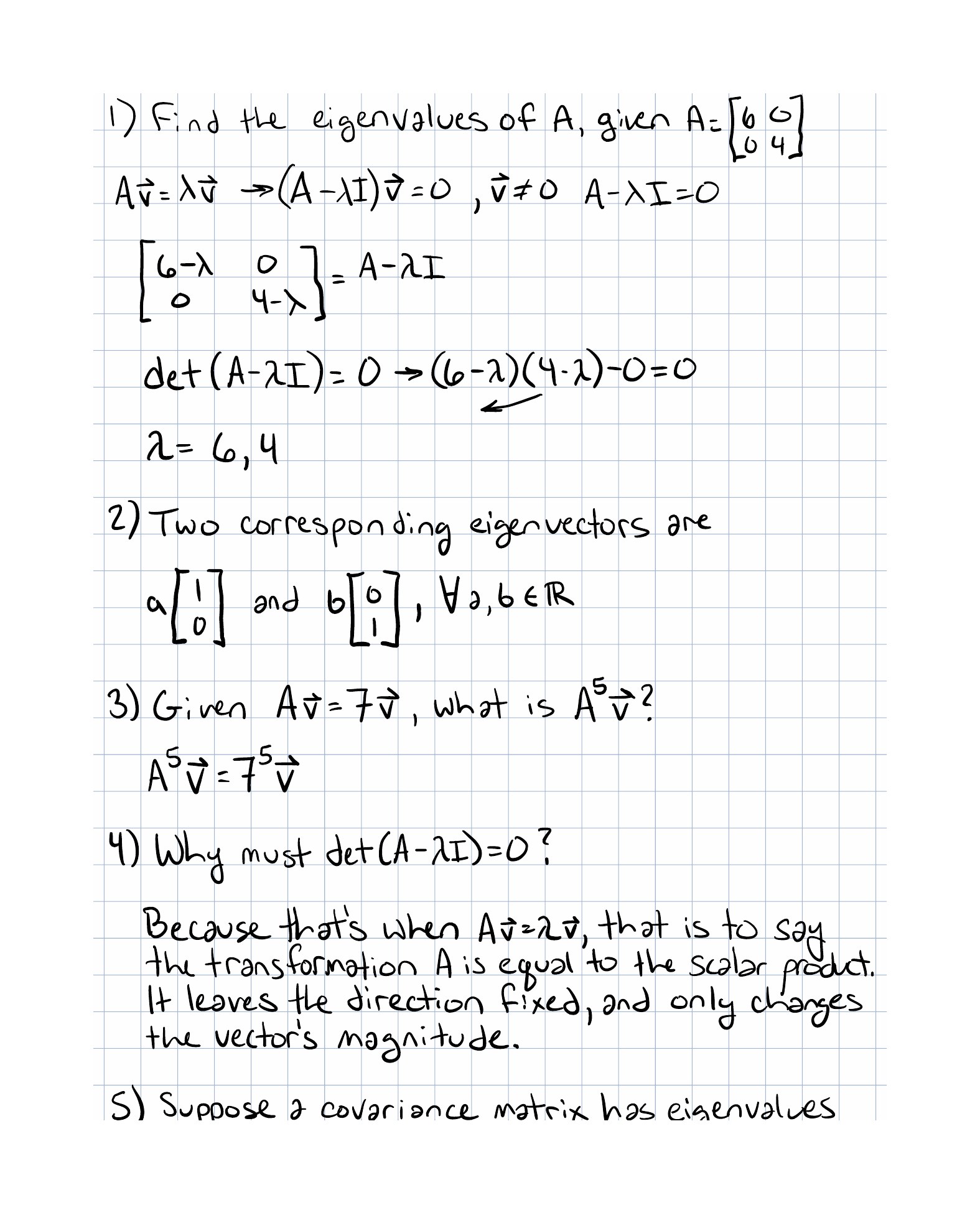
For
$A = \begin{bmatrix} 6 & 0 \\ 0 & 4 \end{bmatrix},$
what are the eigenvalues?
Give one eigenvector for each eigenvalue above.
If $Av = 7v$ , what is $A^5v$ ?
Explain why $det(A - λI) = 0$ must hold if $λ$ is an eigenvalue.
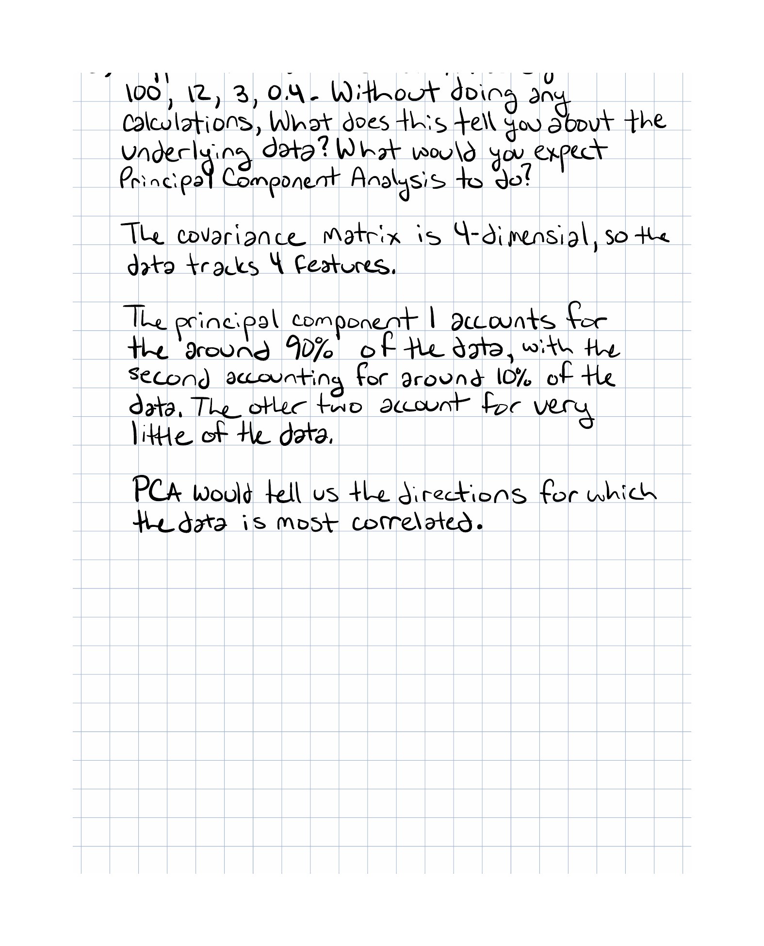
Suppose a covariance matrix has eigenvalues $100$ , $12$ , $3$ , and $0.4$ . What does that suggest about the data, and what would PCA do with it?

Implementation Exercise

Write a TypeScript helper that checks whether a candidate vector is an eigenvector of a 2x2 matrix within a small tolerance.

A useful starting point is:

type Matrix2x2 = [[number, number], [number, number]];
type Vector2 = [number, number];

type EigencheckResult = {
  isEigenvector: boolean;
  eigenvalue: number | null;
  residual: Vector2;
};

The helper should:

compute $Av$ ,
estimate the scalar $λ$ from a nonzero component of $v$ ,
verify whether $Av$ is close to $λv$ ,
return the residual so the caller can inspect the mismatch.

That keeps the exercise close to the lesson: test the defining equation directly.

Reflection Questions

What changed in your mind when you first saw $Av = λv$ ?
Why is repeated application of a matrix easier along an eigenvector?
Which step in the derivation made the determinant appear naturally?
Where do eigenvectors act as a coordinate system for a problem?
Which part of the notation still wants a local reminder?

Next Lesson

Next: Change of Basis.

The bridge is direct: once you know a matrix has preferred directions, the next question is how to re-express a vector in a different basis so those directions become easier to work with.

Completed Exercises

Handwritten work submitted after completing this lesson.