Lesson 7: Change of Basis | Mathematics of AI

Goal

Understand that a vector does not change when we change basis; only its coordinates do.

By the end of the lesson, you should be able to explain why orthonormal bases are especially convenient and why an orthogonal matrix can be inverted by transposition.

Motivation

The data usually does not care which coordinate system we pick.

We care.

When the coordinates are poorly chosen, a problem can look messy. When the coordinates line up with the geometry, the same problem can become almost trivial.

That is why basis changes matter in machine learning. PCA is one of the clearest examples: it looks for a better coordinate system, not a different dataset.

Prerequisites

Lesson 1: Vectors.
Lesson 2: Matrices as Linear Transformations.
Lesson 3: Matrix Multiplication.
Lesson 5: Inverse Matrices.
Lesson 6: Eigenvectors and Eigenvalues.
The dot product and the idea of perpendicular vectors.

Notation / Symbol Table

Symbol	Plain-English name	Meaning
$e_1, e_2$	standard basis vectors	The usual coordinate axes in $\mathbb{R}^2$ .
$u_1, u_2$	alternate basis vectors	A different set of coordinate directions for the same space.
$Q$	orthogonal matrix	A matrix whose columns are orthonormal basis vectors.
$Q^T$	transpose of Q	For orthogonal $Q$ , the inverse transformation.
$u \cdot v$	dot product	A test for orthogonality.
$I$	identity matrix	The matrix that leaves vectors unchanged.

Core Ideas

Coordinates are not the vector

If you write

v = \begin{bmatrix} 3 \\ 4 \end{bmatrix},

those numbers are coordinates in the standard basis.

They are not properties of the vector itself.

If we change the basis, the coordinates change too, even though the vector is the same geometric object.

That distinction is the heart of the lesson.

A basis is a measuring system

The standard basis is

e_1 = \begin{bmatrix} 1 \\ 0 \end{bmatrix}, \qquad e_2 = \begin{bmatrix} 0 \\ 1 \end{bmatrix}.

Any vector in $\mathbb{R}^2$ can be written as a linear combination of those two directions.

But we could choose a different pair, such as

u_1 = \begin{bmatrix} 1 \\ 1 \end{bmatrix}, \qquad u_2 = \begin{bmatrix} 1 \\ -1 \end{bmatrix}.

If the two new directions are linearly independent, they also form a basis.

The vector did not change.

Only the coordinate system did.

Orthogonal and orthonormal bases

Two vectors are orthogonal if their dot product is zero:

u \cdot v = 0.

If we also normalize them to have length 1, the basis is orthonormal.

Orthogonal bases are nice because the coordinate directions do not interfere with one another.

Orthonormal bases are even better because the algebra becomes especially clean.

Orthogonal matrices

If the columns of a matrix $Q$ form an orthonormal basis, then

Q^TQ = I.

Q^{-1} = Q^T.

That is a major simplification.

Instead of solving for an inverse with general linear algebra, we can just transpose.

Change of basis formula

If the columns of $Q$ are the new basis vectors, then the coordinates of a vector $x$ in that basis are

Q^Tx

when $Q$ is orthogonal.

If the basis is not orthonormal, you still change coordinates, but you need the full inverse instead of the transpose.

That is why orthonormal bases are such a sweet spot.

Why this matters for PCA

Eigenvectors of a covariance matrix are perpendicular.

After normalization, they become an orthonormal basis.

If you place them into a matrix $Q$ , then $Q^Tx$ expresses each data point in a new coordinate system where the directions are uncoupled and ordered by variance.

That is the coordinate system PCA wants.

Worked Example

Let

Q = \frac{1}{\sqrt{2}} \begin{bmatrix} 1 & 1 \\ 1 & -1 \end{bmatrix}.

The columns of $Q$ are orthonormal, so $Q^{-1} = Q^T$ .

Take

x = \begin{bmatrix} 3 \\ 4 \end{bmatrix}.

Convert the coordinates:

Q^Tx = \frac{1}{\sqrt{2}} \begin{bmatrix} 1 & 1 \\ 1 & -1 \end{bmatrix} \begin{bmatrix} 3 \\ 4 \end{bmatrix} = \frac{1}{\sqrt{2}} \begin{bmatrix} 7 \\ -1 \end{bmatrix}.

So the same geometric vector now has coordinates

\begin{bmatrix} 7 / \sqrt{2} \\ -1 / \sqrt{2} \end{bmatrix}

in the new basis.

Nothing moved in space.

Only the description changed.

If we want to recover the original coordinates, we multiply by $Q$ :

Q(Q^Tx) = x.

That is the benefit of orthogonality: the forward and backward conversions are cheap and exact in theory.

Why This Shows Up In ML

Machine learning is full of latent coordinate systems.

Feature spaces, principal components, embedding spaces, and orthogonal transforms all depend on the same idea:

Sometimes the smartest thing to do is not to change the data, but to change the coordinates.

Orthogonal transforms preserve lengths and angles, so they are numerically stable and geometrically honest.

That is one reason they are so useful in PCA, whitening, numerical linear algebra, and many optimization methods.

Common Confusions

A change of basis does not move the vector in space; it changes the coordinates used to describe it.
Orthogonal does not mean “same as the standard basis.” It means perpendicular.
An orthogonal matrix may include a reflection, not just a pure rotation.
If the basis is not orthonormal, transpose is not enough; you need the inverse.
The vector and its coordinates are related, but they are not the same thing.

Exercises

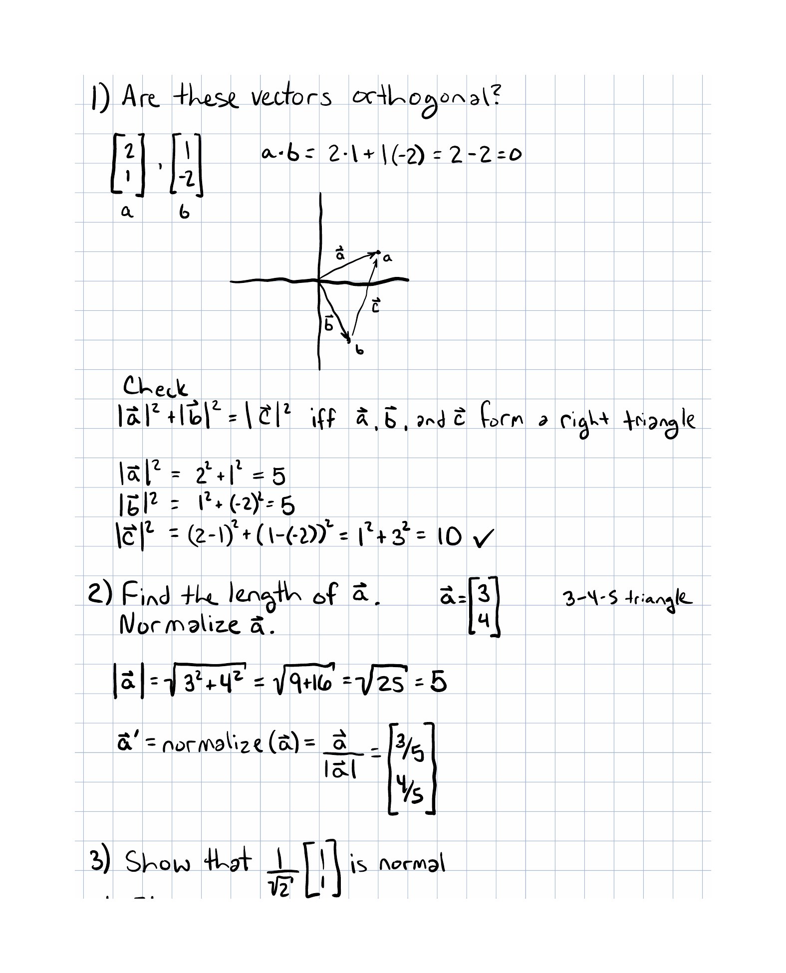
Are these vectors orthogonal?
$\begin{bmatrix} 2 \\ 1 \end{bmatrix}, \quad \begin{bmatrix} 1 \\ -2 \end{bmatrix}$
Find the length of
$\begin{bmatrix} 3 \\ 4 \end{bmatrix}$
and normalize it.
Show that
$\frac{1}{\sqrt{2}} \begin{bmatrix} 1 \\ 1 \end{bmatrix}$
has length 1.
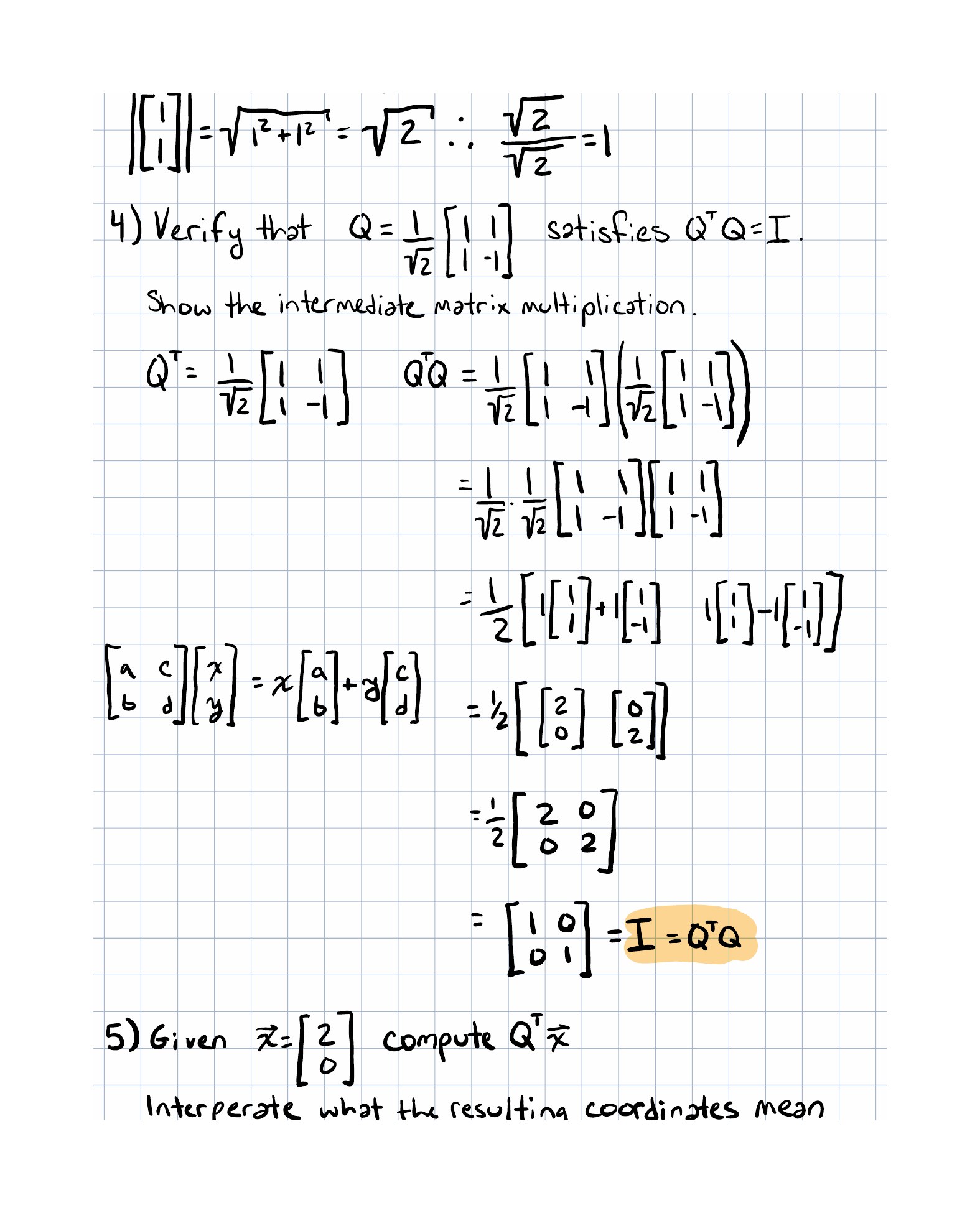
Verify that
$Q = \frac{1}{\sqrt{2}} \begin{bmatrix} 1 & 1 \\ 1 & -1 \end{bmatrix}$
satisfies $Q^TQ = I$ .
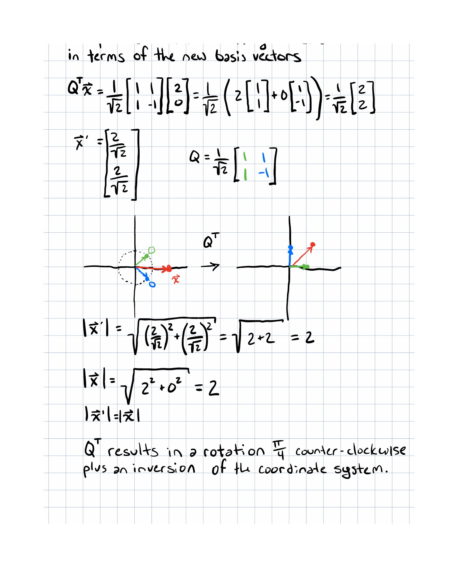
Suppose your data point is
$x = \begin{bmatrix} 2 \\ 0 \end{bmatrix}.$
Compute $Q^Tx$ using the same matrix $Q$ above, and interpret the resulting coordinates.

Implementation Exercise

Write a TypeScript helper that converts coordinates between the standard basis and an orthonormal basis.

A small API could look like this:

type Vector2 = [number, number];
type Matrix2x2 = [[number, number], [number, number]];

function multiplyMatrixVector(matrix: Matrix2x2, vector: Vector2): Vector2;
function transpose(matrix: Matrix2x2): Matrix2x2;

Then use those helpers to implement:

toBasis(Q, x) returning $Q^Tx$ ,
fromBasis(Q, coords) returning $Q \cdot coords$ .

The goal is to make the coordinate change explicit instead of magical.

Reflection Questions

What changed when you noticed that coordinates are not the vector itself?
Why does an orthonormal basis make coordinate conversion simpler?
What is the practical advantage of $Q^{-1} = Q^T$ ?
Where in ML would you rather change coordinates than change the data?
Which part of the basis-change story still feels easy to forget?

Next Lesson

Next: Projection.

The bridge is direct: once we know how to express vectors in a basis, we can ask for the closest vector in a subspace, which is projection.

Completed Exercises

Handwritten work submitted after completing this lesson.