Lesson 9: Least Squares | Mathematics of AI

Goal

Understand least squares as the best approximation you can make when an exact solution does not exist.

The key move is to replace “solve the system exactly” with “find the closest point in the model space.”

Motivation

Real data is noisy.

That means the equations we wish were consistent usually are not.

If we insist on exact equality, many modeling problems have no answer at all.

Least squares gives us a sensible replacement: choose the parameters that make the total squared error as small as possible.

That is the backbone of linear regression and a large number of related fitting procedures.

Prerequisites

Lesson 3: Matrix Multiplication.
Lesson 5: Inverse Matrices.
Lesson 7: Change of Basis.
Lesson 8: Projection.
The idea of an overdetermined system.

Notation / Symbol Table

Symbol	Plain-English name	Meaning
$A$	design matrix	The matrix that turns parameters into predictions.
$x$	parameter vector	The coefficients we want to fit.
$b$	observation vector	The data we are trying to match.
$\hat{x}$	least-squares solution	The best-fit parameter vector.
$e$	residual	The difference $b - A\hat{x}$ .
$A^TA$	normal-equation matrix	The square matrix that appears after projecting.
$A^Tb$	projected right-hand side	The data vector expressed in the normal equations.

Core Ideas

When exact solving fails

If you have more equations than unknowns, the system is overdetermined.

That does not mean the problem is meaningless. It means the equations are asking for too much exact agreement.

For noisy data, exact agreement is usually the wrong target.

Least squares as a projection problem

The vector $Ax$ always lives in the column space of $A$ .

If $b$ is not in that space, there is no exact solution to $Ax = b$ .

So we ask for the point in $\mathrm{col}(A)$ closest to $b$ .

That is a projection problem.

The residual

e = b - A\hat{x}

must be orthogonal to every column of $A$ .

The normal equations

Orthogonality to every column means

A^T(b - A\hat{x}) = 0.

Expanding gives

A^TA\hat{x} = A^Tb.

Those are the normal equations.

If the columns of $A$ are linearly independent, then $A^TA$ is invertible and we can solve

\hat{x} = (A^TA)^{-1}A^Tb.

Why this matters

This is the first place where the geometry and the algebra line up perfectly:

the geometry says “project onto the column space”;
the algebra says “solve the normal equations.”

They are the same statement in different languages.

Worked Example

Suppose we want to fit a line

y = ax + b

to the data

(1, 2.1),\ (2, 3.8),\ (3, 6.2),\ (4, 7.9).

The design matrix and target vector are

A = \begin{bmatrix} 1 & 1 \\ 2 & 1 \\ 3 & 1 \\ 4 & 1 \end{bmatrix}, \qquad b = \begin{bmatrix} 2.1 \\ 3.8 \\ 6.2 \\ 7.9 \end{bmatrix}.

The normal equations use

A^TA = \begin{bmatrix} 30 & 10 \\ 10 & 4 \end{bmatrix}, \qquad A^Tb = \begin{bmatrix} 59.9 \\ 20 \end{bmatrix}.

So we solve

\begin{bmatrix} 30 & 10 \\ 10 & 4 \end{bmatrix} \begin{bmatrix} a \\ b \end{bmatrix} = \begin{bmatrix} 59.9 \\ 20 \end{bmatrix}.

The solution is

a = 1.98, \qquad b = 0.05.

So the best-fit line is

y = 1.98x + 0.05.

The residuals are

0.07,\ -0.21,\ 0.21,\ -0.07.

They are small and balanced rather than forced to vanish.

That is what a good least-squares fit looks like.

Why This Shows Up In ML

Least squares is the ancestor of linear regression.

If each row of $A$ describes an example and each entry of $b$ is a target value, then $\hat{x}$ is the parameter vector that best predicts the targets in the least-squares sense.

That matrix form shows up constantly in machine learning papers.

Whenever you see $X^TX$ , a projection problem is usually hiding underneath.

Common Confusions

Least squares does not mean “make every error zero.” It means “minimize the sum of squared errors.”
The residual is orthogonal to the column space, not necessarily to the raw data points.
Overdetermined does not mean impossible; it means exact consistency is unlikely.
$A^TA$ is square, but that does not automatically make it well-conditioned.
The solution is geometric before it is algebraic.

Exercises

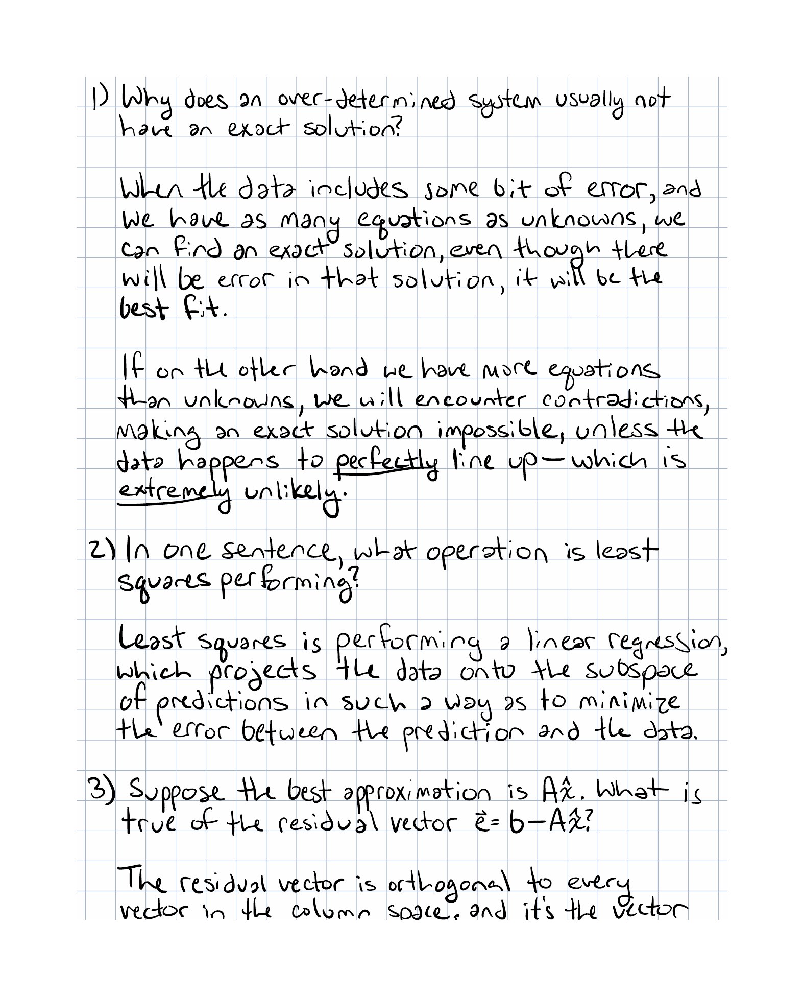
Why does an overdetermined system usually not have an exact solution?
In one sentence, what geometric operation is least squares performing?
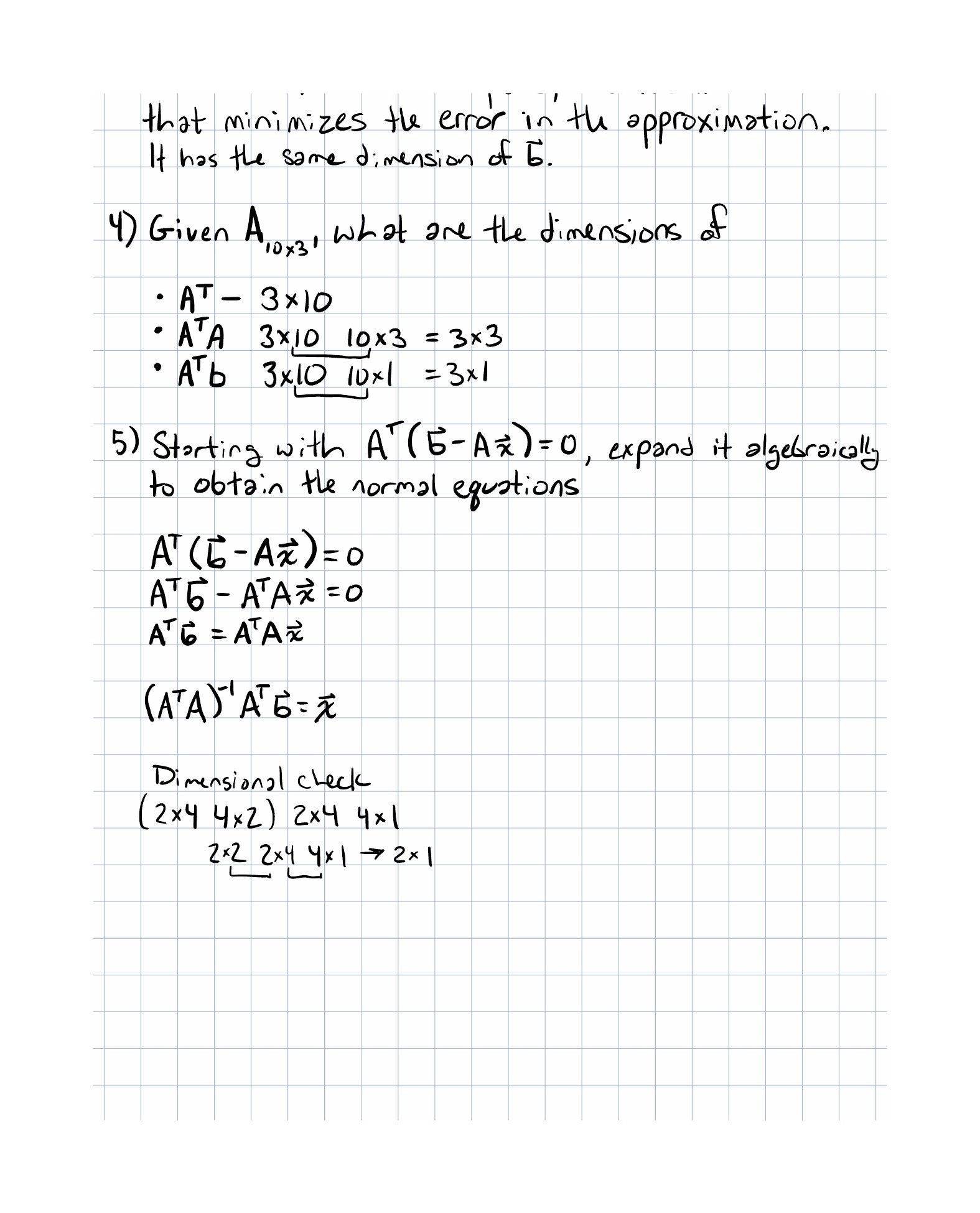
If $\hat{x}$ is the best approximation, what must be true about the residual $e = b - A\hat{x}$ ?
If $A$ is $10 \times 3$ , what are the dimensions of $A^T$ , $A^TA$ , and $A^Tb$ ?
Starting from $A^T(b - Ax) = 0$ , derive the normal equations.

Implementation Exercise

Write a TypeScript helper that fits a line $y = ax + b$ to a set of 2D points using the normal equations.

A simple API could look like this:

type Point = { x: number; y: number };

type LineFit = {
  slope: number;
  intercept: number;
};

function fitLineLeastSquares(points: Point[]): LineFit;

The implementation should:

accumulate the sums needed for $A^TA$ and $A^Tb$ ,
solve the resulting 2x2 system,
return the slope and intercept.

That makes the algebra concrete and keeps the matrix structure visible.

Reflection Questions

What changed when the problem moved from “solve exactly” to “fit best”?
Why does the residual need to be orthogonal to the column space?
Where is the projection hiding inside the normal equations?
Which part of the matrix setup is easiest to forget under time pressure?
What would a noisy dataset look like if a perfect fit existed anyway?

Next Lesson

Next: Singular Value Decomposition.

The bridge is direct: SVD explains the geometry of every matrix, including the ones that are rectangular or rank deficient, and it connects the projection and least-squares ideas to PCA.

Completed Exercises

Handwritten work submitted after completing this lesson.