Goal
Understand the singular value decomposition as a universal description of what a matrix does to space:
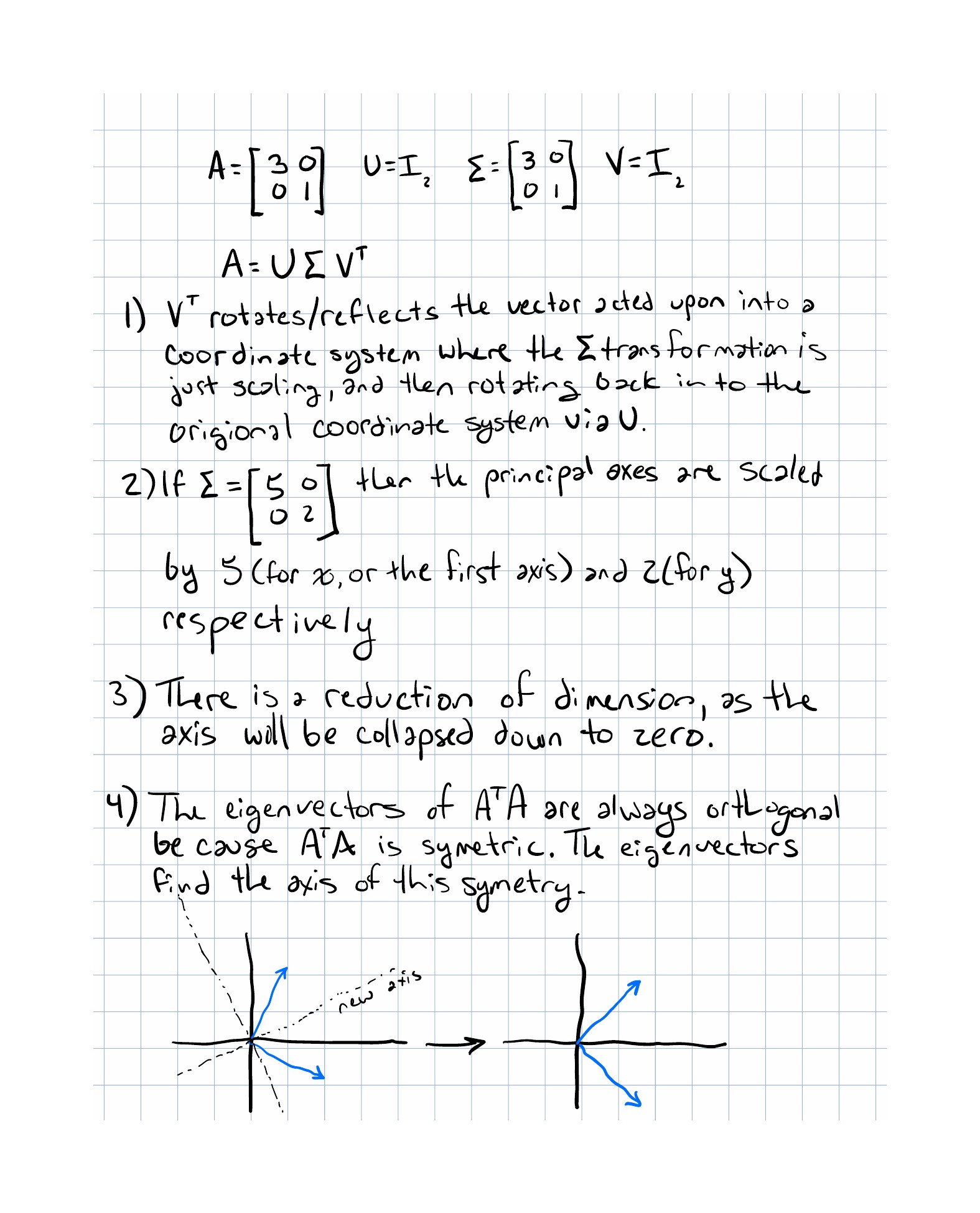
rotate or reflect, stretch independently along orthogonal axes, then rotate or reflect again.
By the end of the lesson, you should be able to read as geometry rather than as a memorized factorization.
Motivation
Eigenvectors work beautifully for some matrices, but not for all matrices.
SVD is the stronger statement.
Every real matrix has an SVD, even if it is rectangular, singular, or awkward.
That is why SVD is one of the most useful theorems in applied linear algebra. It gives a common geometric language for compression, approximation, and dimensionality reduction.
Prerequisites
- Lesson 6: Eigenvectors and Eigenvalues.
- Lesson 7: Change of Basis.
- Lesson 8: Projection.
- Lesson 9: Least Squares.
- The idea of orthogonal matrices and diagonal scaling.
Notation / Symbol Table
| Symbol | Plain-English name | Meaning |
|---|---|---|
| matrix | The linear map being decomposed. | |
| left orthogonal factor | The output-side orthogonal matrix. | |
| diagonal singular-value matrix | The matrix of nonnegative stretch factors. | |
| right orthogonal factor | The input-side orthogonal matrix transpose. | |
| singular value | The i-th nonnegative scale factor. | |
| left singular vector | A column of . | |
| right singular vector | A column of . |
Core Ideas
The factorization
The singular value decomposition writes a matrix as
This is not just a bookkeeping trick.
It is a geometric description of the transformation.
The three stages
Think of the action on a vector in three steps:
- changes coordinates into the matrix’s preferred input basis.
- stretches each coordinate independently.
- rotates or reflects the result into the output orientation.
That is the rotate-stretch-rotate picture.
The preferred basis is determined by the matrix itself, not chosen arbitrarily.
Why the middle matrix is diagonal
The singular values live on the diagonal of .
Because the matrix is diagonal in that middle basis, there is no mixing between coordinates there.
Each axis is scaled independently.
That is exactly the simplification we wanted.
Where the basis comes from
The columns of are the eigenvectors of .
The columns of are the eigenvectors of .
Those matrices are symmetric, so their eigenvectors can be chosen orthonormal.
That orthogonality is what makes the decomposition clean.
Why the squares matter
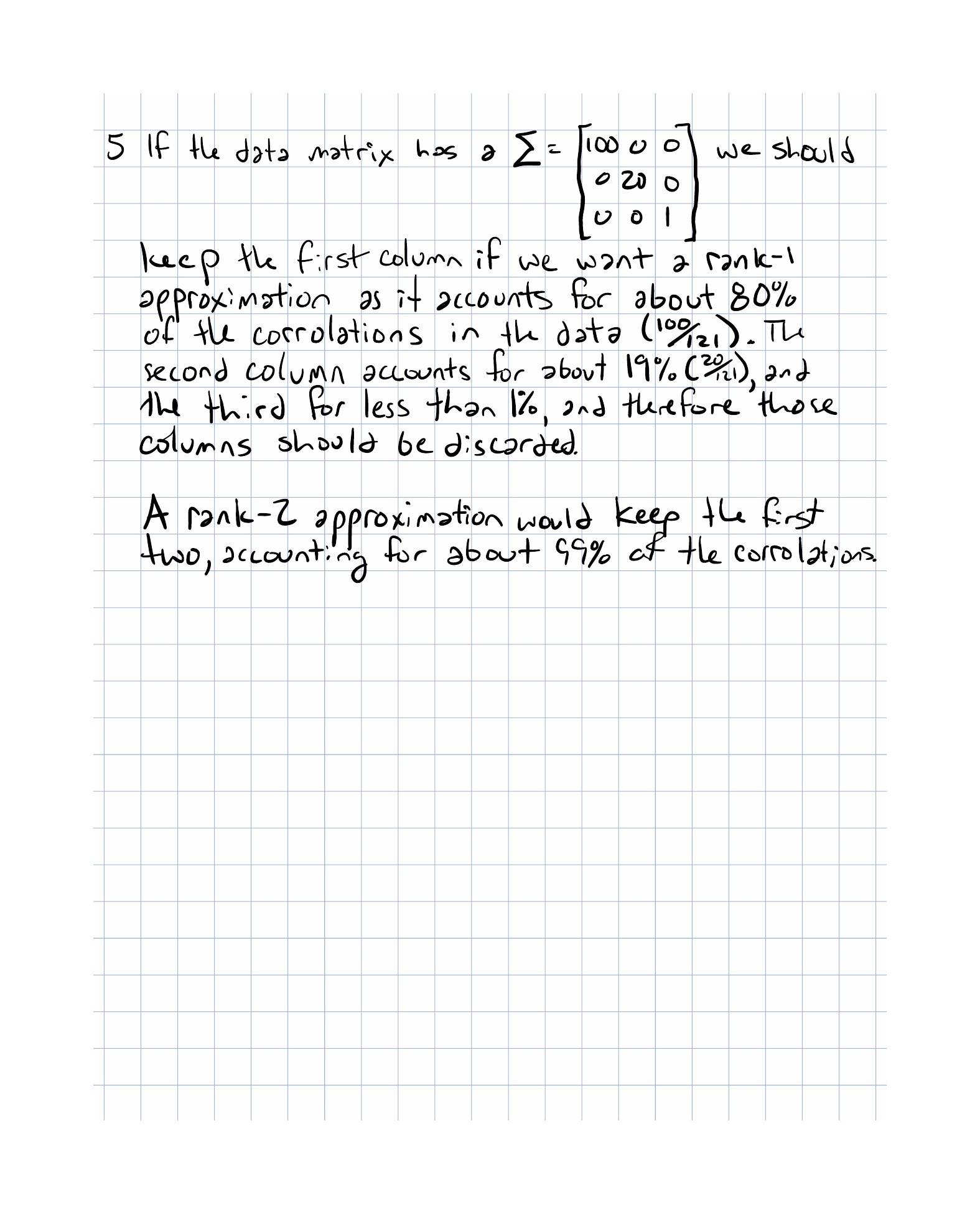
In PCA and related “variance explained” calculations, the important quantity is not but .
Stretch by 10 does not mean “10 times more energy.” It means “100 times more squared energy.”
So if the singular values are , , and , the relative contributions are proportional to
That is the correction that makes PCA and SVD line up with variance.
Worked Example
Start with the simple diagonal matrix
In this case, the SVD is especially simple:
The matrix just stretches the first axis by 5 and the second axis by 2.
If
then
That example is simple, but it shows the meaning of the diagonal middle factor.
Now compare that with a rank-deficient case.
If
then one direction is completely collapsed.
That means the transformation loses a dimension and cannot be inverted.
Energy share example
Suppose the singular values are , , and .
The squared values are
Total energy:
So the first component accounts for about of the energy.
That is why a rank-1 approximation can be so effective when one singular value dominates.
Why This Shows Up In ML
SVD shows up in:
- PCA,
- dimensionality reduction,
- low-rank approximation,
- recommendation systems,
- image compression,
- numerical linear algebra,
- least-squares analysis.
PCA is especially close to SVD.
The singular vectors give the principal directions, and the squared singular values tell you how much variance each direction captures.
That makes SVD the practical engine behind many PCA implementations.
Common Confusions
- does not rotate into the original basis. It rotates into the matrix’s preferred input basis.
- Singular values are not eigenvalues, though they are related through and .
- The values that matter for variance are , not .
- and can include reflections, not only rotations.
- Every real matrix has an SVD, even if it is not square.
Exercises
-
Describe the three stages of the SVD in plain English.
-
If , what happens to a vector on each principal axis?
-
What does a singular value of zero mean geometrically?
-
Why are the eigenvectors of orthogonal?
-
If the singular values are , , and , what fraction of the energy does the first component capture?
Implementation Exercise
Write a TypeScript helper that computes how much variance or energy each singular value contributes.
A useful shape is:
function singularValueEnergyFractions(singularValues: number[]): number[];
function cumulativeEnergy(singularValues: number[], k: number): number;
The implementation should:
- square each singular value,
- sum the squares,
- return each component’s share of the total,
- optionally compute the retained energy for a rank-k approximation.
That exercise reinforces the main SVD lesson: the squares are what matter for explained energy.
Reflection Questions
- What basis is choosing, and why does the matrix prefer it?
- Why does the middle factor have to be diagonal?
- What does a zero singular value do to the dimension of the output?
- Why do the squares matter when talking about explained variance?
- Where in ML does SVD feel like the hidden engine behind another idea?
Next Lesson
Next: Principal Component Analysis.
The bridge is immediate: PCA uses the same geometry as SVD to find the directions of largest variance in data.
Completed Exercises
Handwritten work submitted after completing this lesson.