Lesson 11: Principal Component Analysis

Goal

Understand principal component analysis, or PCA, as a basis change for data: center the data cloud, find the directions where it spreads out the most, rotate into that coordinate system, and optionally keep only the most informative directions.

Motivation

A dataset with many features can be hard to think about directly.

For a person, features might include height, weight, arm span, and shoe size. For an image, each pixel can become a coordinate. In either case, the raw coordinate system is usually not the most revealing one.

PCA asks a better question:

Which directions in this space actually carry most of the variation?

If the data mostly lies near a lower-dimensional shape, PCA gives a coordinate system aligned with that shape. That makes the structure easier to see, easier to compress, and often easier to model.

Prerequisites

Lesson 6: Eigenvectors and Eigenvalues.
Lesson 7: Change of Basis.
Lesson 8: Projection.
Lesson 10: Singular Value Decomposition.

Notation / Symbol Table

Symbol	Plain-English name	Meaning
$x_i$	sample vector	The $i$ -th data point.
$\mu$	mean vector	The average of all sample vectors.
$x_i - \mu$	centered sample	Sample $i$ after subtracting the mean.
$X$	centered data matrix	Matrix with centered samples as rows.
$\Sigma$	covariance matrix	Describes spread and co-variation of the centered data.
$v_1, v_2, \ldots$	principal directions	Orthogonal directions ordered by captured variance.
$\lambda_1, \lambda_2, \ldots$	principal variances	Variance captured along the corresponding principal directions.
$z$	PCA coordinates	Coordinates after projecting onto the principal-component basis.

The first principal component is the direction $v_1$ that maximizes projected variance subject to having unit length. Later components do the same job under an orthogonality constraint.

Core Ideas

A data cloud usually has a shape

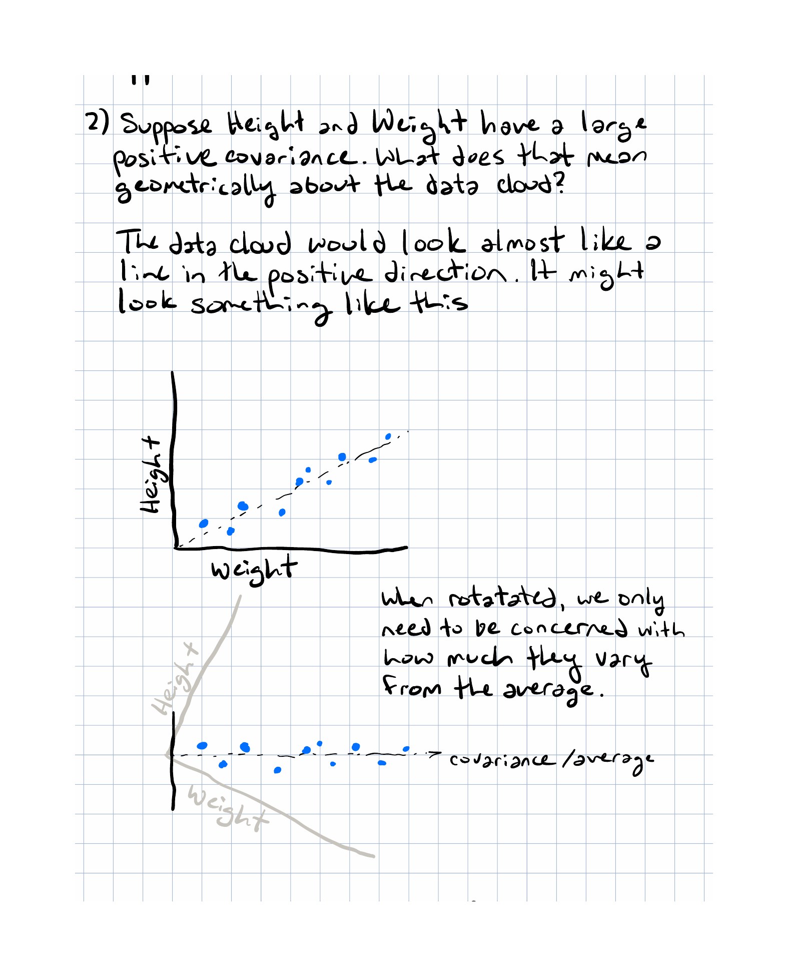
If you plot height against weight, the points do not usually fill the entire plane. They often stretch along a diagonal direction. That means the original coordinates contain redundancy.

PCA looks for coordinates that match the shape of the data cloud instead of the naming scheme of the original features.

Center the data first

Before looking for important directions, subtract the mean:

x_i' = x_i - \mu.

This moves the cloud so it is centered at the origin.

Centering matters because PCA is about variation, not absolute position. We want to know how the data spreads around its average.

Principal components are directions of maximum variance

Pick any unit vector $u$ . If we project the centered data onto $u$ , some choices of $u$ create a wide spread and some create a narrow spread.

PCA chooses the direction with the widest spread first. That direction is the first principal component.

Then it chooses the next orthogonal direction with the largest remaining spread, and so on.

This gives a new orthogonal basis:

v_1, v_2, \ldots, v_n.

Covariance turns the shape into a matrix

The covariance matrix records both variance and co-variation:

\Sigma = \frac{1}{n} X^T X

when $X$ is the centered data matrix with one sample per row.

The diagonal entries tell us variance along the original coordinates. The off-diagonal entries tell us how coordinates move together.

PCA works because the eigenvectors of $\Sigma$ are the natural axes of this spread.

Eigenvectors and singular vectors are telling the same story

X = U \Sigma_{\text{svd}} V^T,

then

X^T X = V \Sigma_{\text{svd}}^2 V^T.

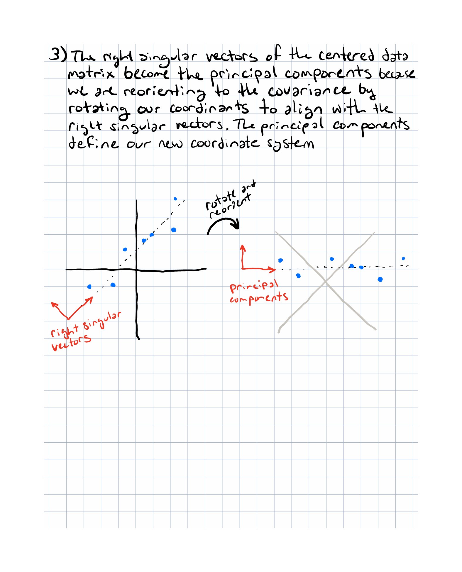
So the right singular vectors of the centered data matrix are exactly the principal directions. The squared singular values determine how much variance lives along each direction.

That is why practical PCA implementations usually use SVD instead of explicitly building the covariance matrix first.

Dimensionality reduction is projection with judgment

Once the principal directions are ordered by importance, we can keep only the first few:

z = V_k^T (x - \mu),

where $V_k$ contains the first $k$ principal directions.

This is just projection into a better basis. The point is not that the dropped directions are mathematically meaningless. The point is that they may contribute very little useful variation.

Worked Example

Consider a centered two-dimensional dataset whose covariance matrix is

\Sigma = \begin{bmatrix} 9 & 6 \\ 6 & 4 \end{bmatrix}.

This matrix says three things immediately:

The first coordinate has variance $9$ .
The second coordinate has variance $4$ .
The positive off-diagonal entries show that the two coordinates tend to increase together.

Now notice that

\Sigma \begin{bmatrix} 3 \\ 2 \end{bmatrix} = \begin{bmatrix} 39 \\ 26 \end{bmatrix} = 13 \begin{bmatrix} 3 \\ 2 \end{bmatrix}.

So $\begin{bmatrix} 3 \\ 2 \end{bmatrix}$ is an eigenvector with eigenvalue $13$ .

That means the first principal direction points along the vector $(3, 2)$ , and the variance along that direction is $13$ .

In plain English: the data cloud is longest along the diagonal line with slope about $2/3$ . If we rotate into that basis, one coordinate carries almost all the visible structure.

Why This Shows Up In ML

PCA appears in machine learning because many datasets have correlated or redundant features.

Common uses include:

dimensionality reduction before downstream modeling;
denoising by discarding low-variance directions;
visualization of high-dimensional data in two or three coordinates;
compression of images, embeddings, or tabular features;
decorrelation as a preprocessing step for classical ML pipelines.

The deeper reason is geometric: many models work better when the coordinate system reflects the actual structure of the data.

Exercises

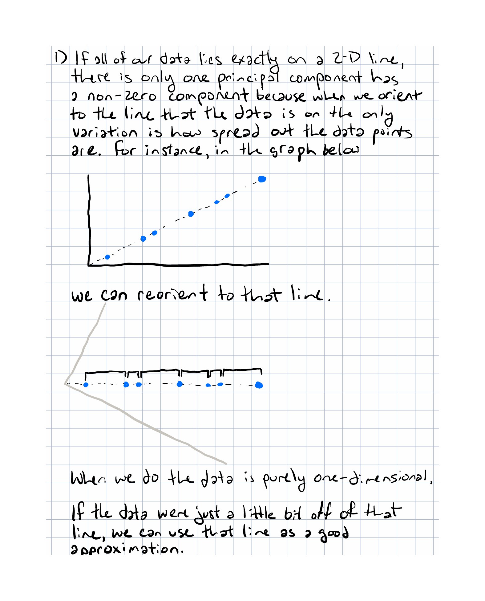
Suppose every point in a two-dimensional dataset lies exactly on a single line through the mean. How many principal components have non-zero variance, and why?
A dataset has two features with large positive covariance. What does that say about the shape and orientation of the point cloud?
Explain, in your own words, why centering the data is necessary before computing principal components.
Why do the right singular vectors of the centered data matrix become the principal-component directions?

Implementation Exercise

Write a TypeScript helper that:

computes the mean of each feature;
centers the dataset;
computes the covariance matrix for a small two-dimensional dataset;
projects each centered point onto the first principal direction.

For a toy dataset, hard-code a small covariance matrix or use a tiny eigensolver for the $2 \times 2$ case. The goal is not numerical sophistication. The goal is to see the whole PCA pipeline as data transformation plus change of basis.

Reflection Questions

Which part of PCA feels most geometric to you: centering, rotating, or projecting?
What does it mean to say that the original features are redundant?
Why is keeping the first few principal components a modeling choice rather than a theorem?
If you had to explain PCA to a programmer, would you describe it as compression, basis change, or shape discovery?

Completed Exercises

Handwritten work submitted after completing this lesson.