Lesson 12: Covariance | Mathematics of AI

Goal

Understand covariance as a measurement of how two variables vary together, and understand the covariance matrix as the object that captures the shape, scale, and orientation of a data cloud.

Motivation

PCA tells us to compute eigenvectors of the covariance matrix. This lesson explains why that advice makes sense.

If variance tells us how spread out one variable is, covariance tells us how two variables move together. Once we collect all those pairwise relationships into a matrix, the matrix starts behaving like a geometric summary of the dataset.

Prerequisites

Lesson 6: Eigenvectors and Eigenvalues.
Lesson 10: Singular Value Decomposition.
Lesson 11: Principal Component Analysis.

Notation / Symbol Table

Symbol	Plain-English name	Meaning
$x_i$	x sample	The $i$ -th observed value of the first variable.
$y_i$	y sample	The $i$ -th observed value of the second variable.
$\mu_x$	x mean	Average of the x-values.
$\mu_y$	y mean	Average of the y-values.
$\operatorname{Var}(X)$	variance	Spread of one variable around its mean.
$\operatorname{Cov}(X, Y)$	covariance	How two variables move together around their means.
$\Sigma$	covariance matrix	Matrix collecting variances and pairwise covariances.

For two variables, covariance is

\operatorname{Cov}(X, Y) = \frac{1}{n} \sum_{i=1}^{n} (x_i - \mu_x)(y_i - \mu_y).

Core Ideas

Variance is spread of one variable

Variance measures how far values typically sit from their mean:

\operatorname{Var}(X) = \frac{1}{n} \sum_{i=1}^{n} (x_i - \mu_x)^2.

The square does two jobs:

positive and negative deviations do not cancel;
larger deviations count more heavily.

Covariance generalizes variance

Covariance uses the same idea, but with two variables:

\operatorname{Cov}(X, Y) = \frac{1}{n} \sum_{i=1}^{n} (x_i - \mu_x)(y_i - \mu_y).

Interpretation:

positive covariance means the variables tend to rise and fall together;
negative covariance means one tends to rise when the other falls;
covariance near zero means there is no strong linear relationship.

Variance is just the special case

\operatorname{Var}(X) = \operatorname{Cov}(X, X).

The covariance matrix records the shape of the cloud

For two coordinates, the covariance matrix is

\Sigma = \begin{bmatrix} \operatorname{Var}(X) & \operatorname{Cov}(X, Y) \\ \operatorname{Cov}(Y, X) & \operatorname{Var}(Y) \end{bmatrix}.

This matrix tells us:

how wide the cloud is;
how tall the cloud is;
how tilted the cloud is.

That is why covariance is the bridge from raw data to geometry.

Symmetry is not an accident

Because real-number multiplication commutes,

(x_i - \mu_x)(y_i - \mu_y) = (y_i - \mu_y)(x_i - \mu_x),

\operatorname{Cov}(X, Y) = \operatorname{Cov}(Y, X).

That is why every covariance matrix is symmetric.

Once symmetry appears, eigenvectors become natural again. Symmetric matrices have orthogonal eigenvectors, and those eigenvectors become the principal axes of the data cloud.

Covariance and centered data matrices

If $A$ is the centered data matrix with one sample per row, then

\Sigma = \frac{1}{n} A^T A.

So the covariance matrix is not a mysterious new object. It is a familiar linear-algebra construction: multiply centered data by its transpose, then average.

This is the exact reason PCA and SVD fit together so cleanly.

Worked Example

Suppose

\Sigma = \begin{bmatrix} 9 & 6 \\ 6 & 4 \end{bmatrix}.

Read it entry by entry:

$\operatorname{Var}(X) = 9$ , so the first coordinate has more spread than the second.
$\operatorname{Var}(Y) = 4$ , so the second coordinate is less spread out.
$\operatorname{Cov}(X, Y) = 6$ , so the coordinates tend to increase together.

Geometrically, the cloud is stretched along a positively sloped diagonal direction. It is not aligned with the original axes.

That is exactly the situation where PCA helps: rotate into the natural axes of the covariance matrix instead of keeping the original feature axes.

Why This Shows Up In ML

Covariance appears throughout machine learning because models care about structure, not just isolated features.

It helps us:

understand feature redundancy;
diagnose scale and correlation in tabular data;
motivate PCA and whitening;
describe Gaussian distributions;
reason about conditioning in optimization.

A covariance matrix is one of the first compact summaries that tells you what a dataset is doing geometrically.

Exercises

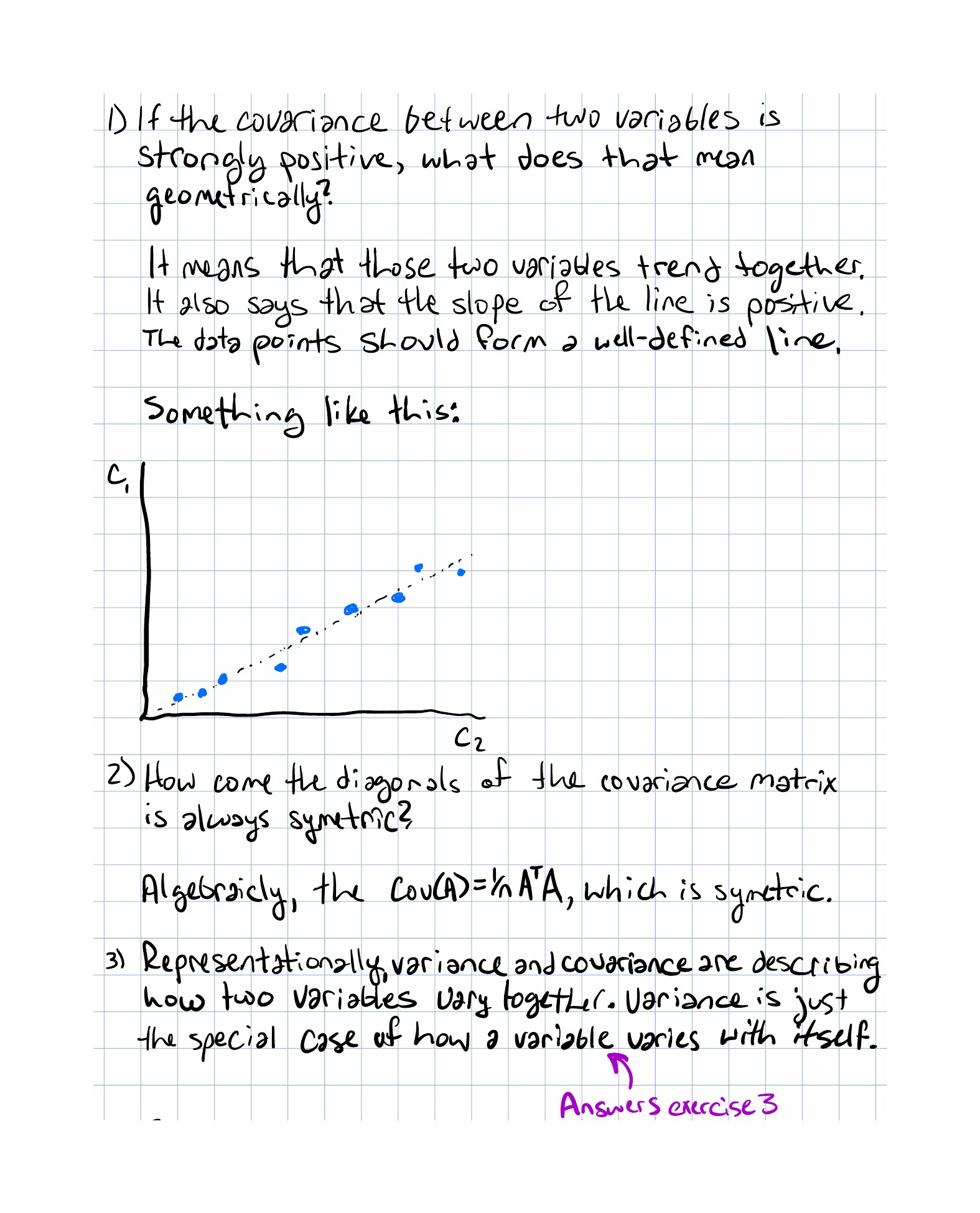
If two variables have large positive covariance, what should the point cloud look like?
Why are the diagonal entries of a covariance matrix always variances?
Why must the covariance matrix be symmetric?
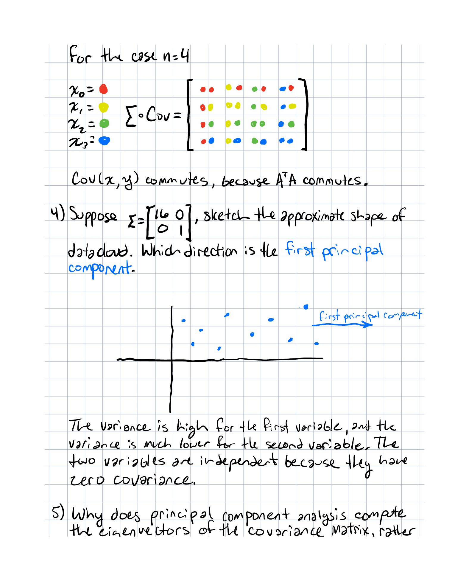
If

\Sigma = \begin{bmatrix} 16 & 0 \\ 0 & 1 \end{bmatrix},

what does the cloud look like, and which direction is the first principal component?

Zero covariance means the variables are uncorrelated. Why does that not automatically imply independence?

Implementation Exercise

Implement a TypeScript function that takes an array of two-dimensional samples and returns:

the mean of each coordinate;
the centered samples;
the $2 \times 2$ covariance matrix.

Then print the matrix for one dataset whose coordinates are visibly correlated and one whose coordinates are not. Compare the off-diagonal entries.

Reflection Questions

When you look at an off-diagonal covariance entry, do you think “formula” or “tilt of the cloud” first?
Why is covariance the right object for explaining PCA?
What is the cleanest difference between covariance near zero and true statistical independence?
If you changed coordinate systems, what would stay the same: the matrix entries, the geometry, or both?

Completed Exercises

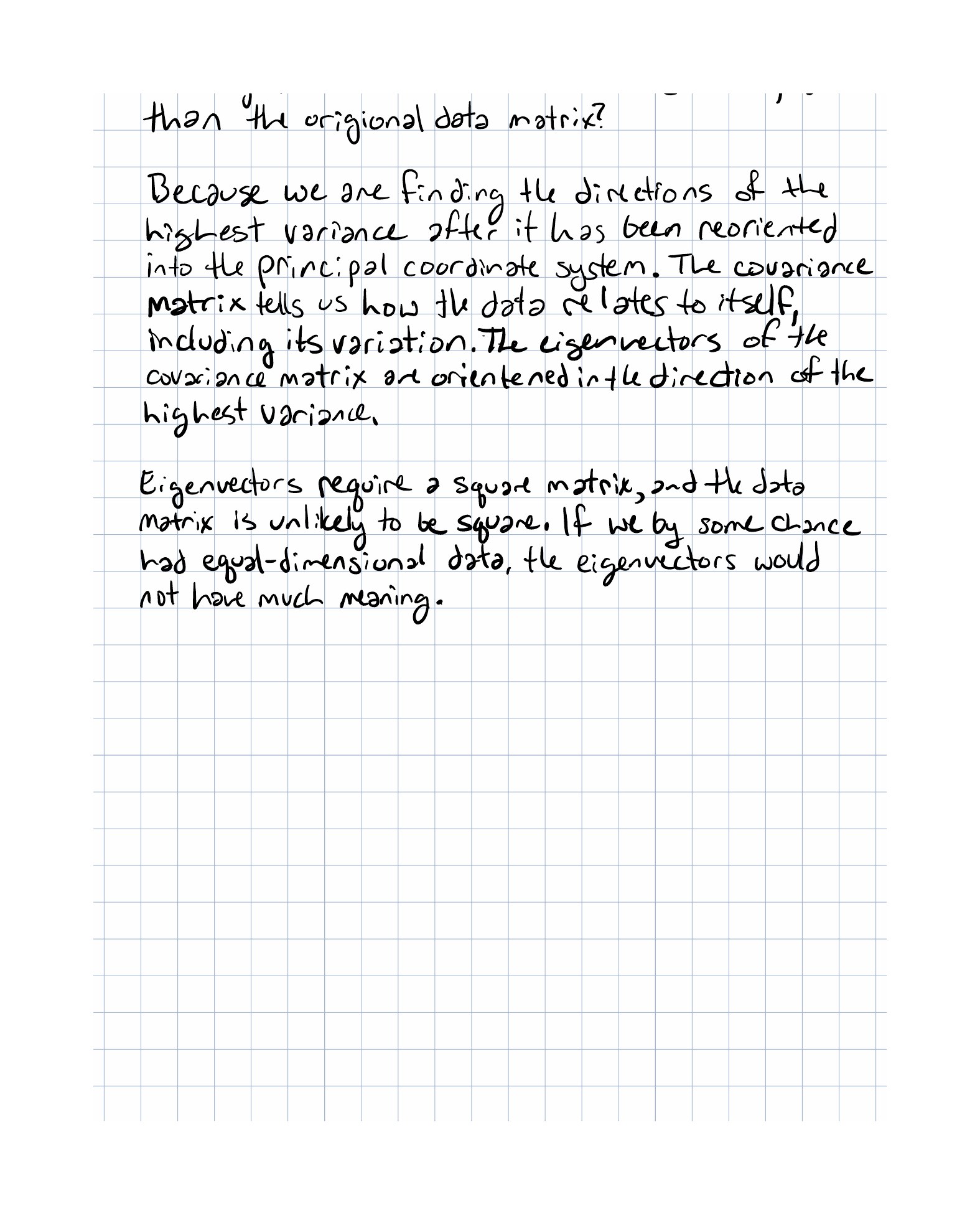
Handwritten work submitted after completing this lesson.