Lesson 13: Probability as Linear Algebra

Goal

Understand probability as a continuation of the linear-algebra story: random variables behave like vectors, expectation behaves like a linear functional, and covariance behaves like a weighted dot product after centering.

Motivation

Machine learning uses probability constantly, but the formulas become much easier to manage when they are tied back to familiar objects.

This lesson gives a unifying view:

a random variable is a function;
expectation is an averaging operator;
variance and covariance are geometric measurements in a vector space of random variables.

That perspective makes the later probability lessons feel less like a branch change and more like the same ideas in new clothing.

Prerequisites

Lesson 11: Principal Component Analysis.
Lesson 12: Covariance.

Notation / Symbol Table

Symbol	Plain-English name	Meaning
$\Omega$	sample space	Set of all possible outcomes.
$\omega$	outcome	One element of the sample space.
$X(\omega)$	random variable value	The number assigned by $X$ to outcome $\omega$ .
$E[X]$	expectation	Weighted average of the values of $X$ .
$\tilde{X}$ or $X̃$	centered random variable	The mean-zero version of $X$ , defined by $X - E[X]$ .
$\operatorname{Var}(X)$	variance	Average squared distance from the mean.
$\operatorname{Cov}(X, Y)$	covariance	Average product of centered values.
$\Sigma$	covariance matrix	Covariance collected across all coordinates of a random vector.

Read $\tilde{X}$ aloud as “X tilde.” In this lesson it always means the centered version of $X$ :

\tilde{X} = X - E[X].

Core Ideas

A random variable is a function

A random variable is not “a random number” in the abstract. It is a function from outcomes to numbers:

X : \Omega \to \mathbb{R}.

For a die roll, one random variable might return the face value. Another might return $1$ for an odd roll and $0$ for an even roll.

The important point is that the same sample space can support many different random variables.

Expectation is a weighted average

For a discrete variable,

E[X] = \sum_i x_i P(x_i).

Expectation is the center of mass of the distribution, not necessarily a value that the variable ever literally takes.

That is why a fair die has expectation $3.5$ even though no roll produces $3.5$ .

Expectation is linear

Expectation respects linear combinations:

E[aX + bY] = aE[X] + bE[Y].

This is a strong hint that expectation should be treated as a linear map, not only as a recipe.

If you like the programming analogy, expectation is a reducer from a structured random object down to one scalar summary.

Centering puts the mean at zero

Define

\tilde{X} = X - E[X].

Then

E[\tilde{X}] = 0.

This is the same centering step we used with datasets. Probability now inherits the same workflow: first subtract the mean, then measure geometry around that center.

Variance is squared length after centering

Variance can be written as

\operatorname{Var}(X) = E[(X - E[X])^2] = E[\tilde{X}^2].

That is the probability version of squared length. If the centered variable usually stays close to zero, the variance is small. If it often wanders far away, the variance is large.

Covariance is a weighted dot product

Covariance is

\operatorname{Cov}(X, Y) = E[(X - E[X])(Y - E[Y])] = E[\tilde{X}\tilde{Y}].

Compare that with a dot product:

a \cdot b = \sum_i a_i b_i.

The structure is the same except that probability adds weights through expectation. That is why covariance behaves so much like an inner product and why the covariance matrix acts like a Gram matrix.

The covariance matrix is an averaged outer product

For a random vector $X$ with mean $\mu$ ,

\Sigma = E[(X - \mu)(X - \mu)^T].

This is the probabilistic version of multiplying centered data by its transpose and averaging. Once you write it this way, PCA looks almost inevitable.

Worked Example

Let a discrete random variable take values

1,\ 3,\ 5

with equal probability.

First compute the expectation:

E[X] = \frac{1 + 3 + 5}{3} = 3.

Now center the values:

\tilde{X} \in \{-2, 0, 2\}.

Then compute the variance:

\operatorname{Var}(X) = E[\tilde{X}^2] = \frac{(-2)^2 + 0^2 + 2^2}{3} = \frac{8}{3}.

This example is small, but it shows the whole pipeline clearly:

define a variable;
average it with expectation;
center it;
square the centered values;
take expectation again.

Why This Shows Up In ML

Machine learning constantly averages over data, noise, and uncertainty.

This point of view shows up when we:

compute average loss over a dataset;
measure variance of errors or features;
build Gaussian models from means and covariances;
define correlations, principal directions, and whitened coordinates;
treat gradients, losses, and predictions as random quantities over sampled data.

The practical win is that probability stops feeling like isolated formulas. It becomes geometry plus averaging.

Exercises

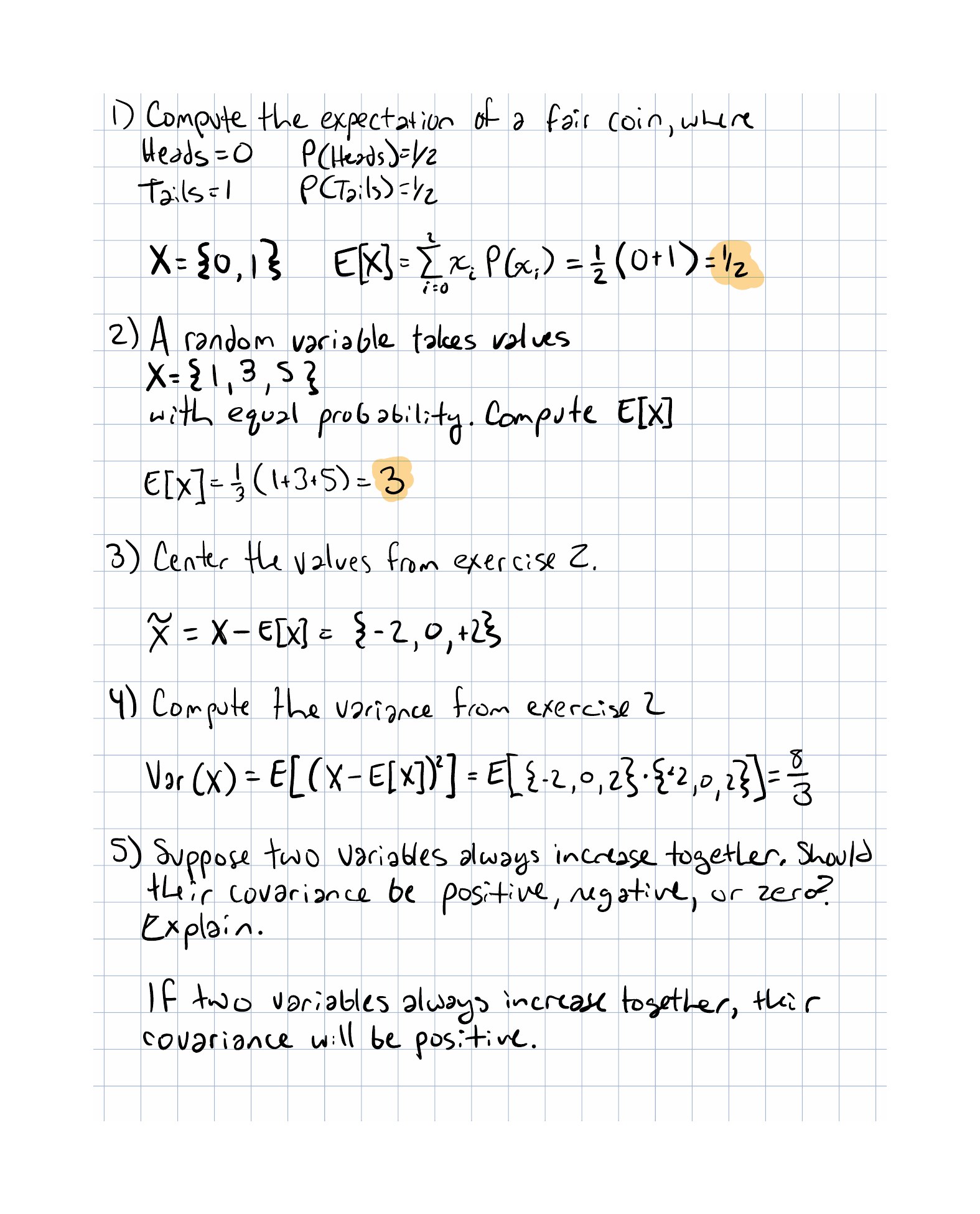
A fair coin uses Heads $= 1$ and Tails $= 0$ . Compute $E[X]$ .
For the variable taking values $1, 3, 5$ with equal probability, compute the centered values again without looking back.
Using the same variable, recompute $\operatorname{Var}(X)$ and say which step turns a list of numbers back into one scalar.
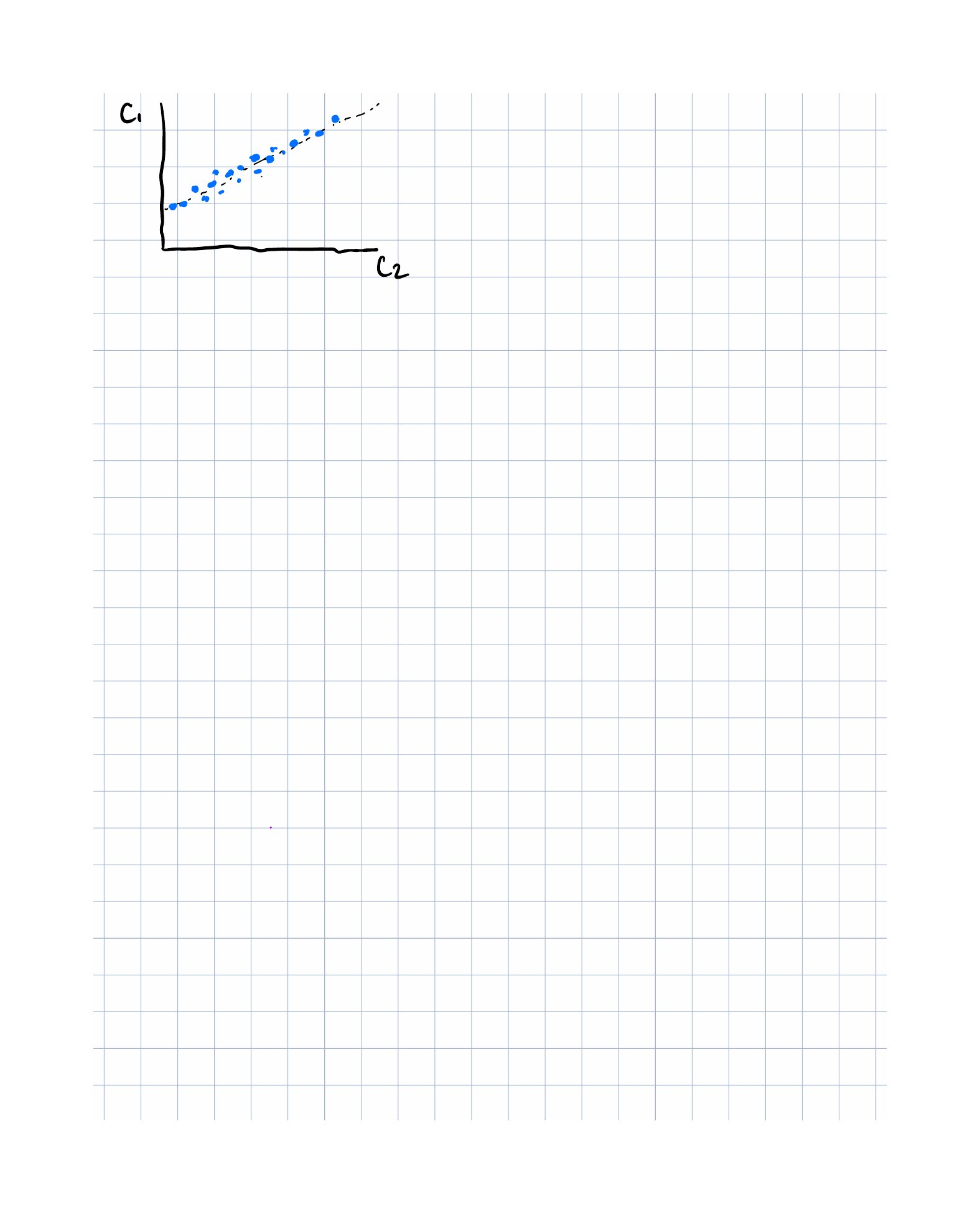
If two centered random variables are usually positive together or negative together, should their covariance be positive, negative, or near zero?
Explain why expectation is a linear map in one sentence and one equation.

Implementation Exercise

Represent a discrete distribution in TypeScript as an array of objects like:

type WeightedValue = {
  value: number;
  probability: number;
};

Then implement helpers for:

expectation;
centering a discrete random variable;
variance.

Use .reduce for the weighted sums so the code mirrors the mathematical definition.

Reflection Questions

Did it help to think of a random variable as a function instead of as a “random number”?
Which feels clearer: variance as a formula or variance as squared distance from the mean?
What does expectation do that centering and squaring do not?
When you see covariance now, do you read it more like a statistic or more like a weighted inner product?

Completed Exercises

Handwritten work submitted after completing this lesson.