Lesson 14: Covariance Geometry

Goal

Understand covariance as geometry: once variables are centered, covariance behaves like an inner product, correlation behaves like cosine, PCA becomes diagonalization, and whitening becomes a rotate-and-rescale change of coordinates.

Motivation

The previous lesson showed that probability can be written in linear-algebra language. This lesson tightens that connection.

Instead of thinking of covariance as just another formula, we will treat it as the structure that gives random variables lengths, angles, and orthogonality. Once that clicks, several later ideas stop feeling unrelated.

Prerequisites

Lesson 12: Covariance.
Lesson 13: Probability as Linear Algebra.

Notation / Symbol Table

Symbol	Plain-English name	Meaning
$\tilde{X}$ or $X̃$	centered $X$	The mean-zero version of random variable $X$ .
$\tilde{Y}$ or $Ỹ$	centered $Y$	The mean-zero version of random variable $Y$ .
$\operatorname{Cov}(X, Y)$	covariance	Inner-product-like pairing of centered random variables.
$\operatorname{Var}(X)$	variance	Covariance of $X$ with itself.
$\rho(X, Y)$	correlation	Normalized covariance, analogous to cosine.
$\Sigma$	covariance matrix	Gram matrix built from pairwise covariances.
$V \Lambda V^T$	eigendecomposition	Rotation into principal directions followed by axis scaling.
$\Lambda^{-1/2}$	whitening scale	Rescales principal directions to unit variance.

We will use

\langle X, Y \rangle = E[\tilde{X}\tilde{Y}] = \operatorname{Cov}(X, Y)

as the key bridge between probability and geometry.

Core Ideas

Centered random variables behave like vectors

Once we center random variables, we can compare them in a way that ignores their means and focuses only on variation.

That makes the pairing

\langle X, Y \rangle = E[\tilde{X}\tilde{Y}]

feel like a dot product:

it is symmetric;
it is linear in each slot;
it is nonnegative when applied to the same variable twice.

So covariance is not only a statistic. It is the geometric structure on this vector space.

Variance is the induced squared norm

If covariance plays the role of inner product, then variance plays the role of squared length:

\operatorname{Var}(X) = \operatorname{Cov}(X, X).

This is the same relationship as

\|v\|^2 = v \cdot v

in ordinary Euclidean space.

Correlation is cosine

Normalize covariance by the lengths of the variables:

\rho(X, Y) = \frac{\operatorname{Cov}(X, Y)} {\sqrt{\operatorname{Var}(X)}\sqrt{\operatorname{Var}(Y)}}.

That is exactly the same pattern as

\cos(\theta) = \frac{x \cdot y}{\|x\|\|y\|}.

So correlation measures angle-like alignment:

$\rho = 1$ means the variables point in the same centered direction;
$\rho = -1$ means they point in opposite directions;
$\rho = 0$ means they are orthogonal in the covariance sense.

The covariance matrix is a Gram matrix

For a random vector with coordinates $X_1, X_2, \ldots, X_n$ , the covariance matrix is

\Sigma_{ij} = \operatorname{Cov}(X_i, X_j).

That means $\Sigma$ is the Gram matrix formed by pairing each coordinate with every other coordinate.

This is why it is symmetric and why diagonalization is the right move. We are looking for the basis in which the geometric structure becomes as simple as possible.

PCA is a rotation into the natural basis

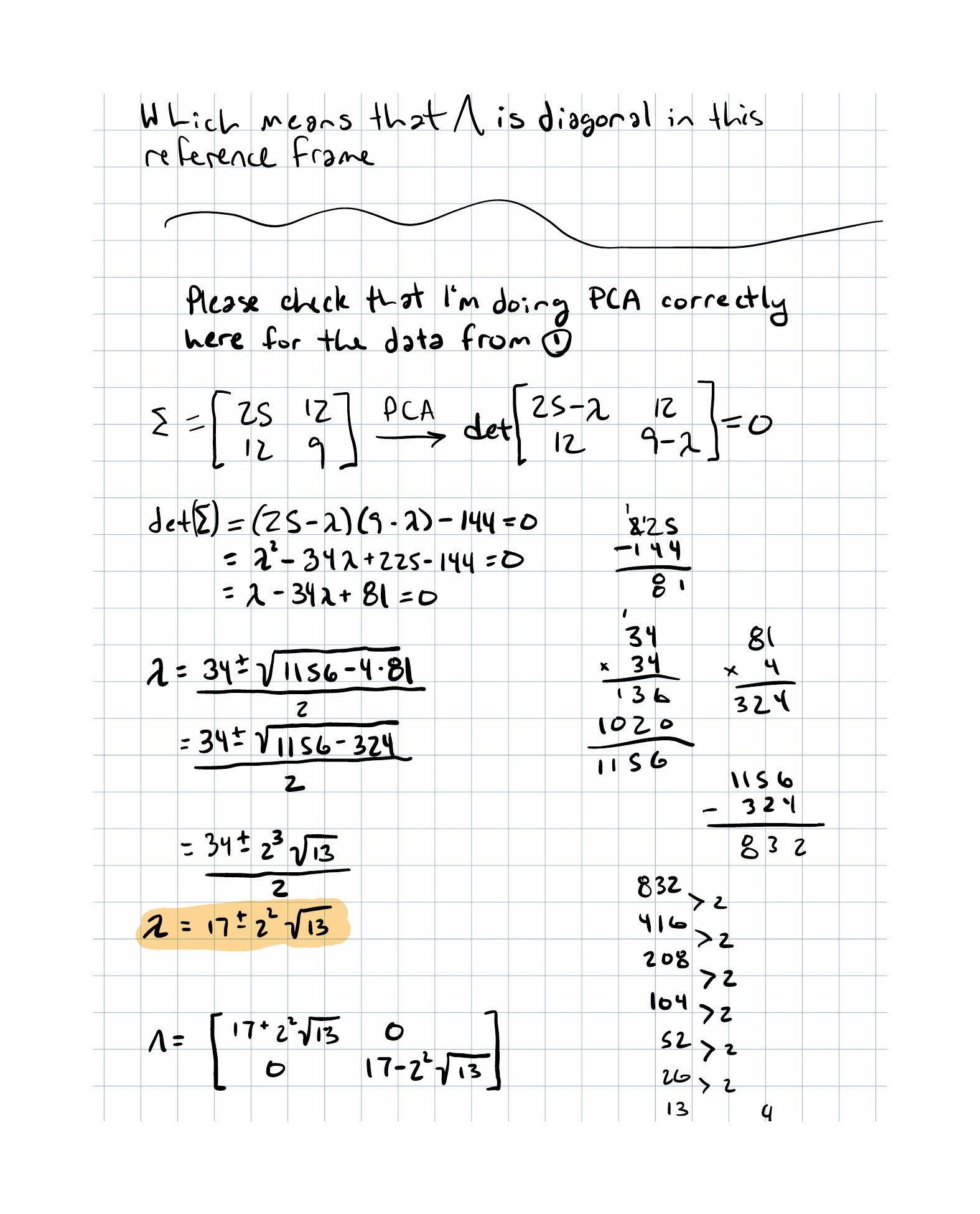
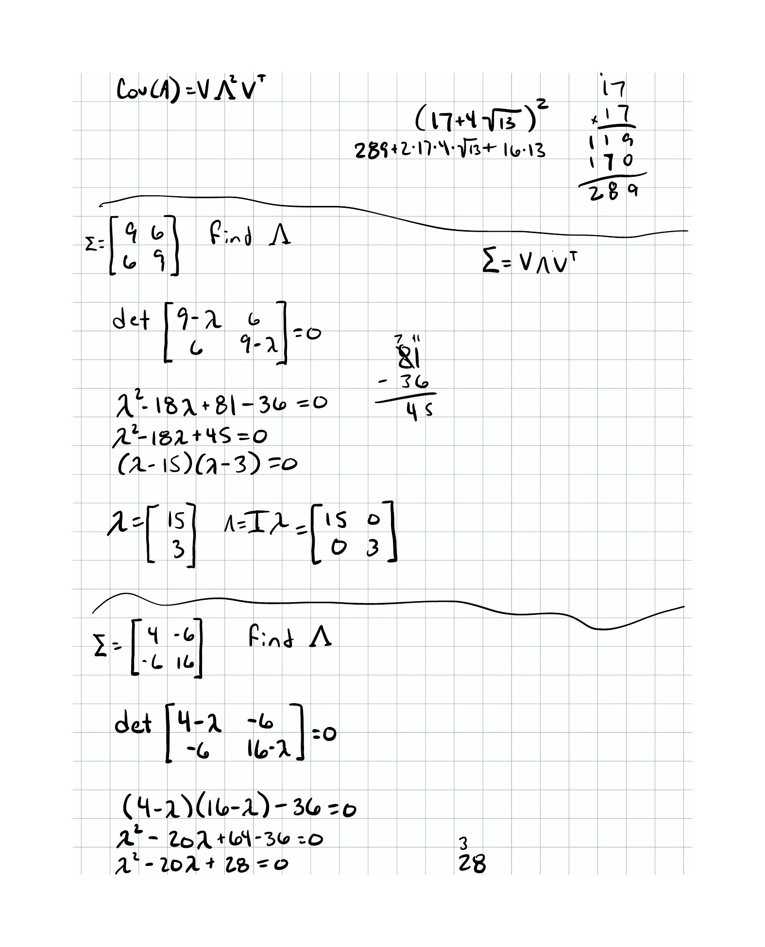
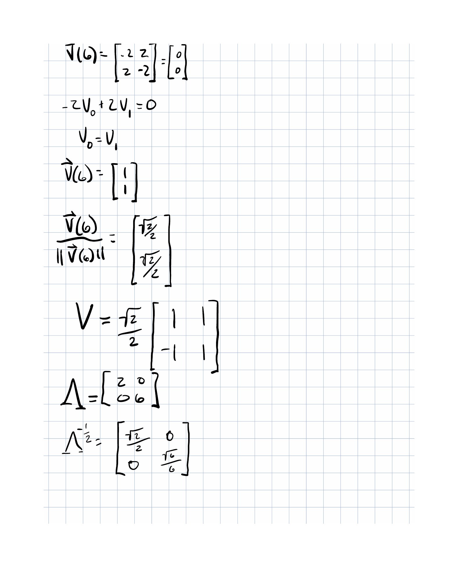
Because covariance matrices are symmetric, they admit an orthogonal eigendecomposition:

\Sigma = V \Lambda V^T.

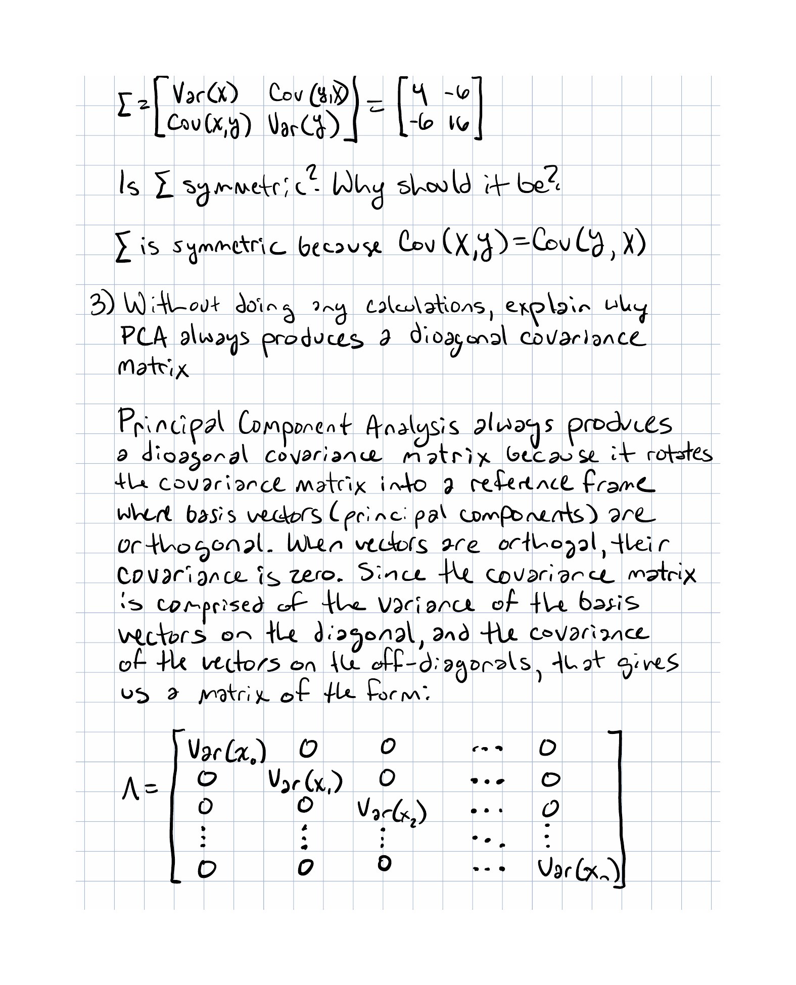
The columns of $V$ are orthogonal principal directions. In that basis, the covariance matrix is diagonal:

V^T \Sigma V = \Lambda.

PCA is not distorting the data. It is choosing the basis in which the covariance geometry is already aligned with the axes.

Whitening rescales the geometry

After PCA, the covariance becomes diagonal but the variances may still be unequal. Whitening applies one more transformation:

z = \Lambda^{-1/2} V^T (x - \mu).

Interpretation:

rotate into principal directions;
divide each direction by its standard deviation.

After whitening, every principal direction has variance $1$ , so the covariance becomes the identity matrix.

Worked Example

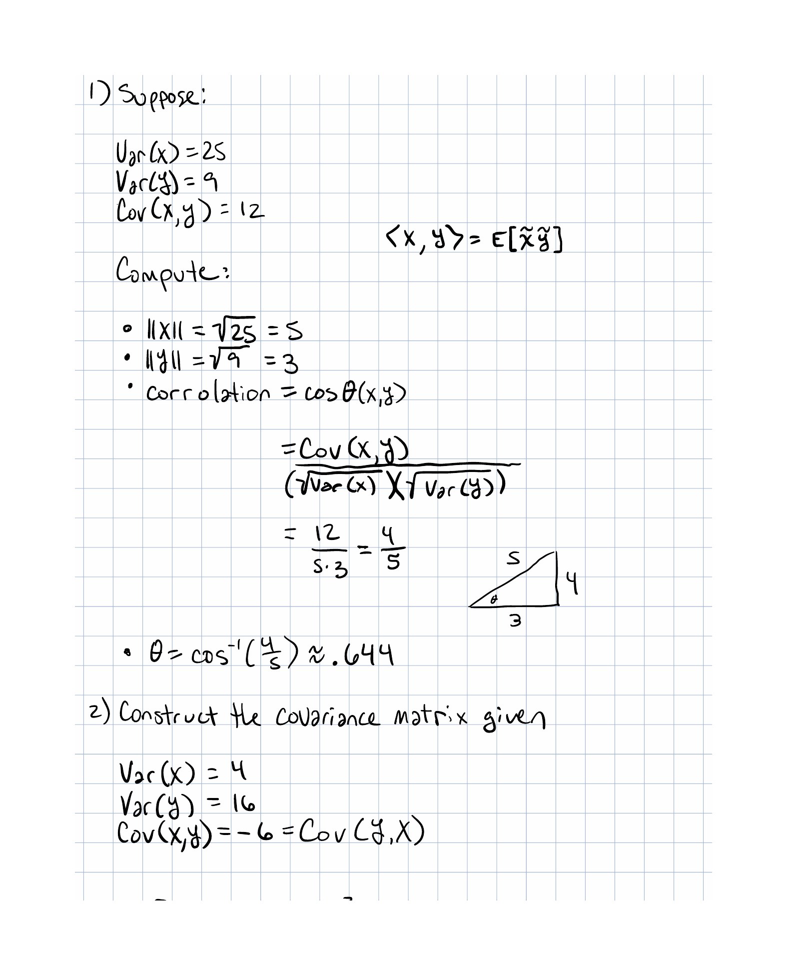
Suppose

\operatorname{Var}(X) = 25,\qquad \operatorname{Var}(Y) = 9,\qquad \operatorname{Cov}(X, Y) = 12.

Then the covariance lengths are

\|X\| = \sqrt{25} = 5,\qquad \|Y\| = \sqrt{9} = 3.

The correlation is

\rho(X, Y) = \frac{12}{5 \cdot 3} = \frac{4}{5}.

So the angle between the centered variables is

\theta = \cos^{-1}\left(\frac{4}{5}\right).

This is the same geometry you already know from a $3$ - $4$ - $5$ triangle: the variables are fairly aligned, but not identical.

That is the payoff of this lesson. A familiar geometric computation now has a statistical interpretation.

Why This Shows Up In ML

This viewpoint matters in machine learning because many standard preprocessing and modeling steps are really geometric operations in disguise.

Examples:

PCA rotates into principal directions.
Whitening removes covariance and standardizes scale.
Feature normalization improves conditioning for optimization.
Latent representations are often compared by covariance structure rather than by raw coordinates.

Once the covariance geometry is visible, many algorithms become easier to motivate and easier to debug.

Exercises

\operatorname{Var}(X) = 4,\qquad \operatorname{Var}(Y) = 16,\qquad \operatorname{Cov}(X, Y) = -6,

compute the correlation and say whether the corresponding angle is acute or obtuse.

Build the covariance matrix from those three quantities. Why must the matrix be symmetric?
Explain, without calculation, why PCA makes the covariance matrix diagonal in the principal-component basis.
In your own words, what does whitening change that PCA alone does not?

Implementation Exercise

Create a tiny TypeScript experiment with a two-dimensional dataset.

Compute the covariance matrix.
Hard-code or compute its orthonormal eigenvectors.
Rotate the centered points into the principal basis.
Rescale each rotated coordinate by the reciprocal of its standard deviation.

Print the covariance before PCA, after rotation, and after whitening. The goal is to see the sequence:

tilted ellipse;
axis-aligned ellipse;
sphere-like cloud.

Reflection Questions

Does correlation feel more natural when read as cosine?
Why is covariance the right notion of orthogonality here instead of ordinary Euclidean dot product on raw coordinates?
Which step in whitening is doing the “rotation” job, and which step is doing the “unit variance” job?
If you had to explain PCA in one sentence now, would you say “maximize variance” or “diagonalize covariance”?

Completed Exercises

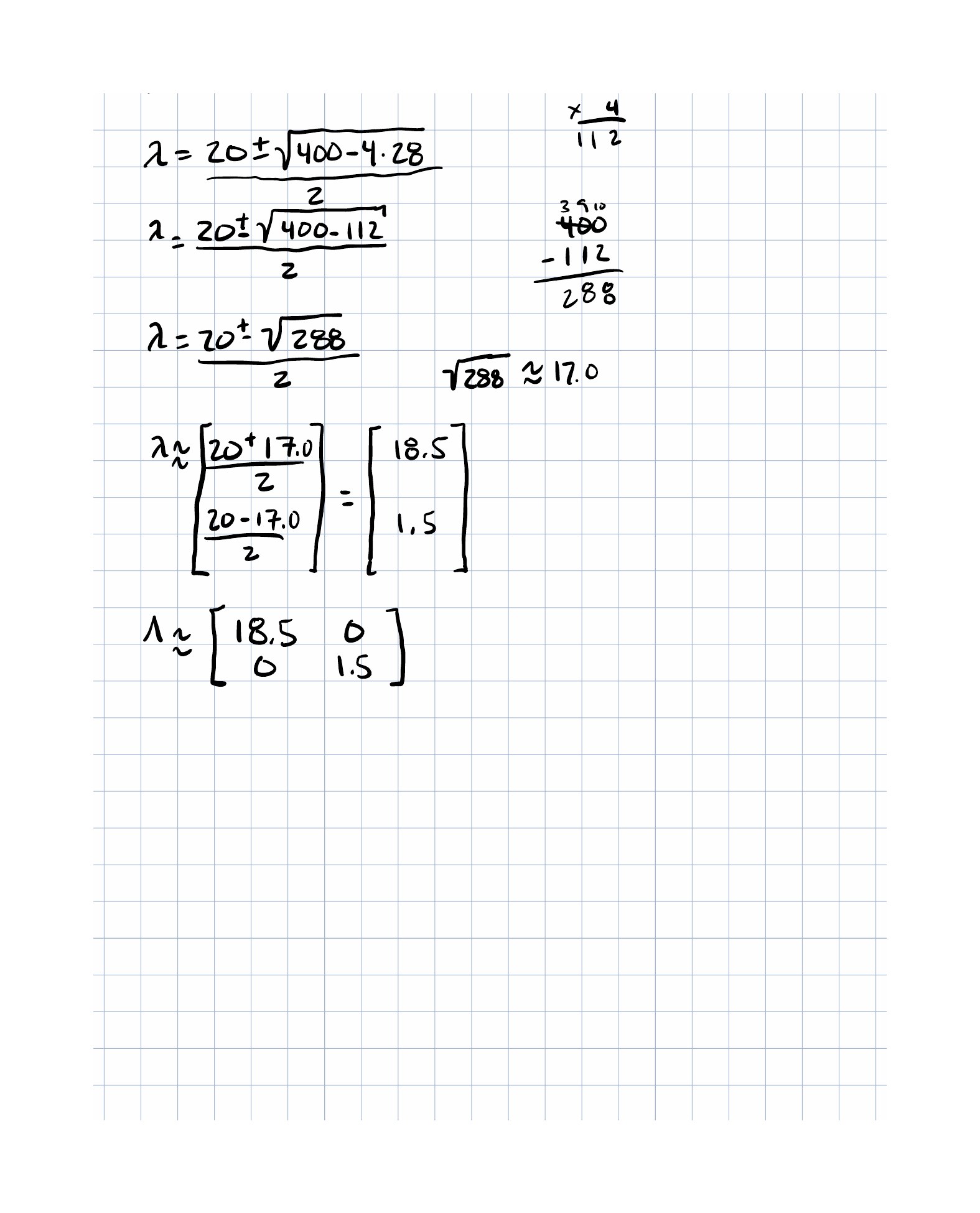
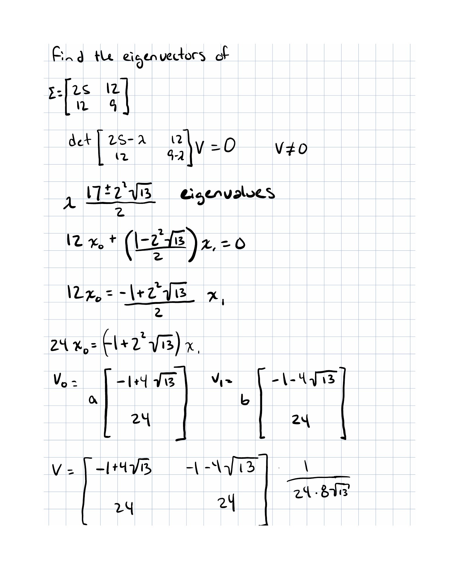
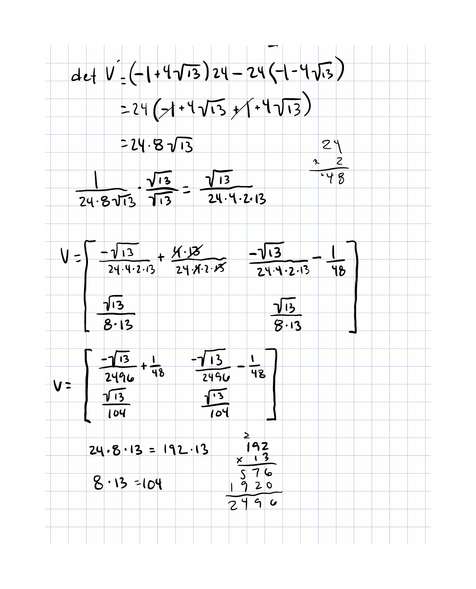
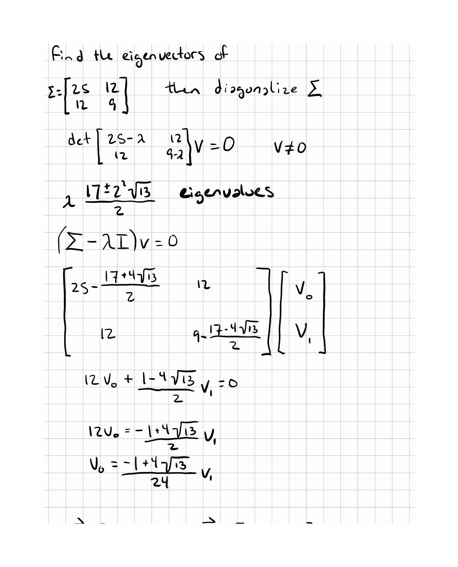
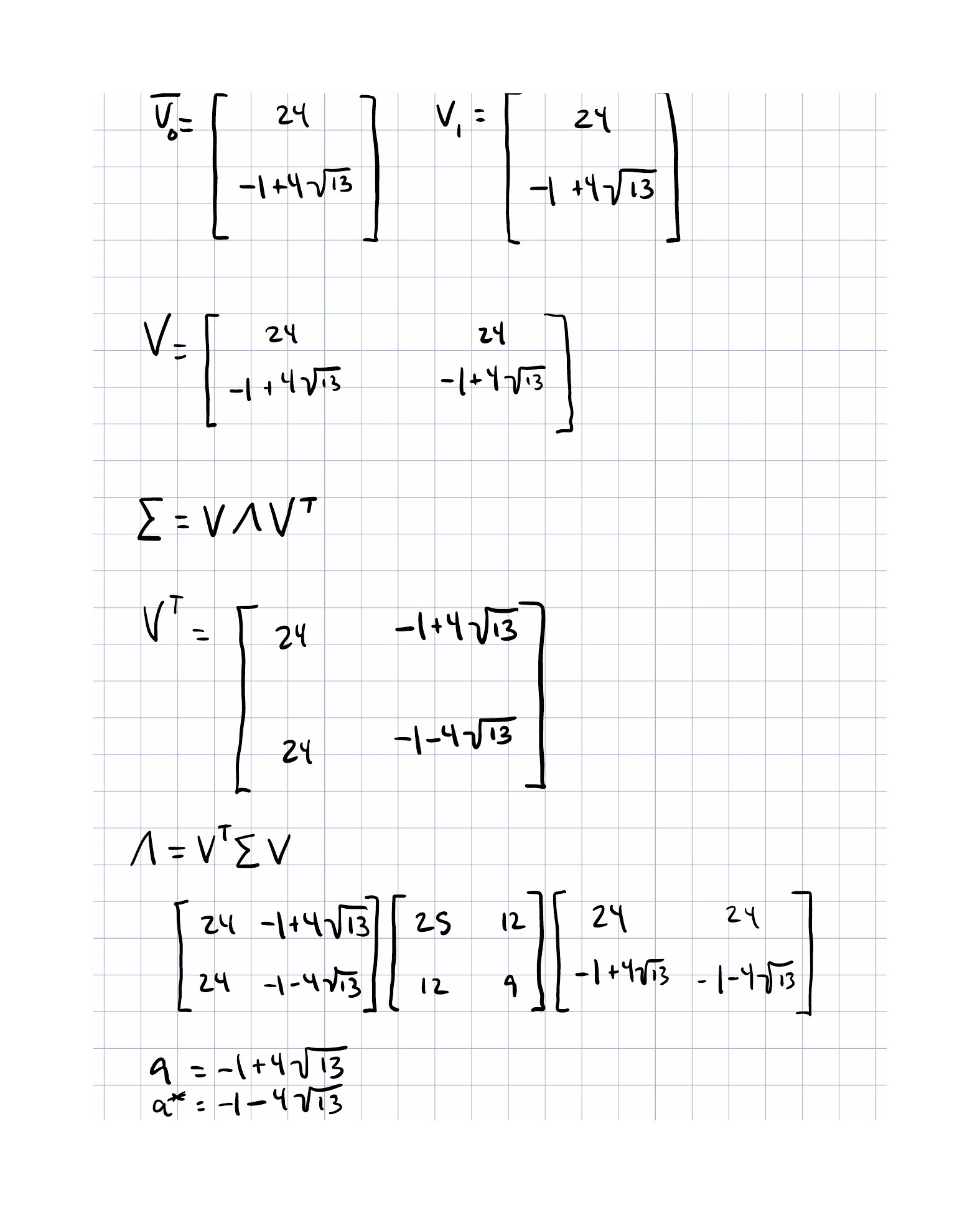
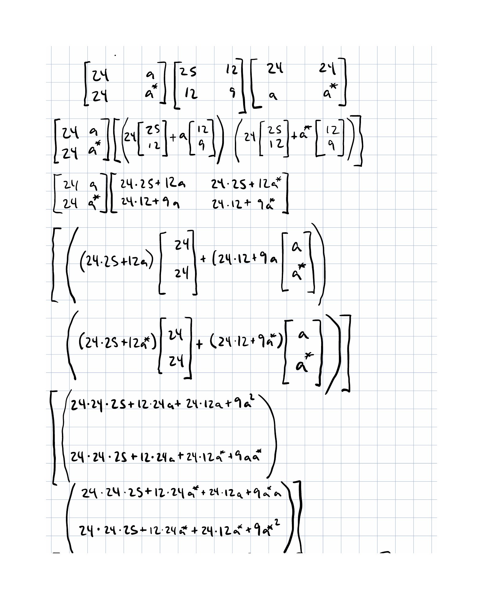
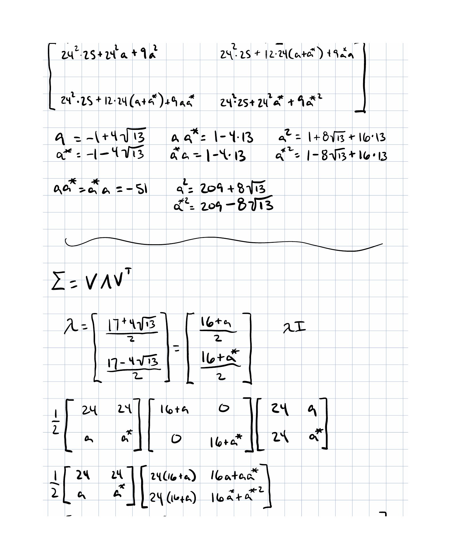
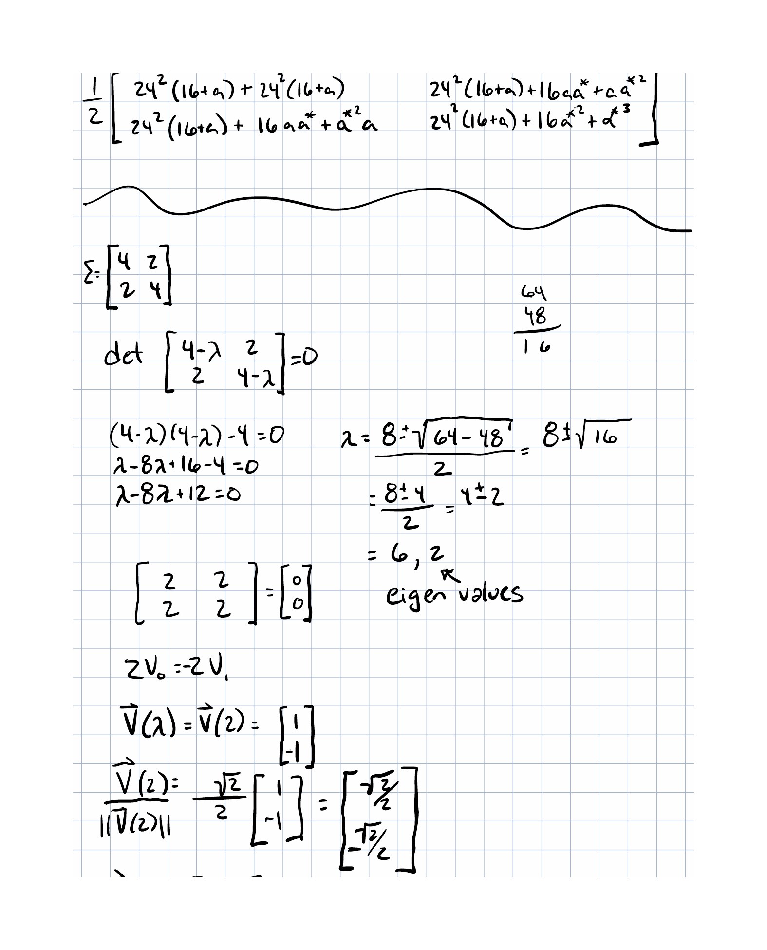
Handwritten work submitted after completing this lesson.