Goal
Understand the multivariate Gaussian as a geometric probability distribution: covariance determines the ellipsoidal shape, the precision matrix determines how distance is measured, and whitening reveals that the distribution is just a spherical Gaussian viewed in transformed coordinates.
Motivation
Many machine learning models assume that some source of noise, uncertainty, or latent variation is Gaussian.
That can feel like a memorized convention until you see the geometry. Once covariance defines an ellipsoid, the multivariate Gaussian becomes the natural probability density built from that geometry.
Prerequisites
- Lesson 12: Covariance.
- Lesson 14: Covariance Geometry.
Notation / Symbol Table
| Symbol | Plain-English name | Meaning |
|---|---|---|
| evaluation point | Point in where the density is evaluated. | |
| mean vector | Center of the Gaussian. | |
| covariance matrix | Describes spread and orientation. | |
| precision matrix | Weights distance by confidence instead of uncertainty. | |
| squared Mahalanobis distance | Distance from to in covariance-scaled geometry. | |
| determinant of covariance | Volume-scaling term used in normalization. | |
| principal variance | Variance along principal direction . | |
| whitened coordinate | Coordinate after removing covariance structure. |
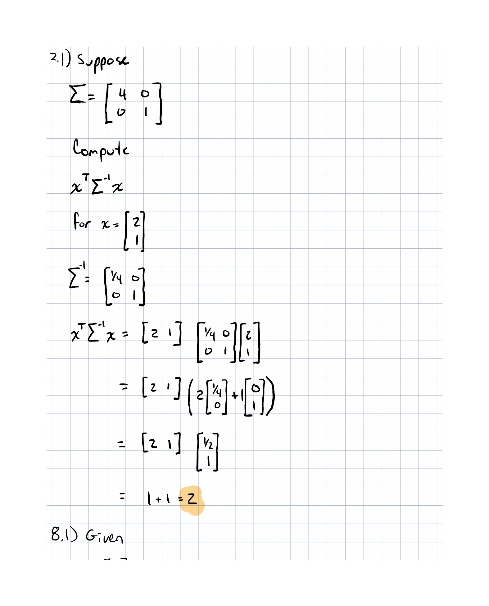
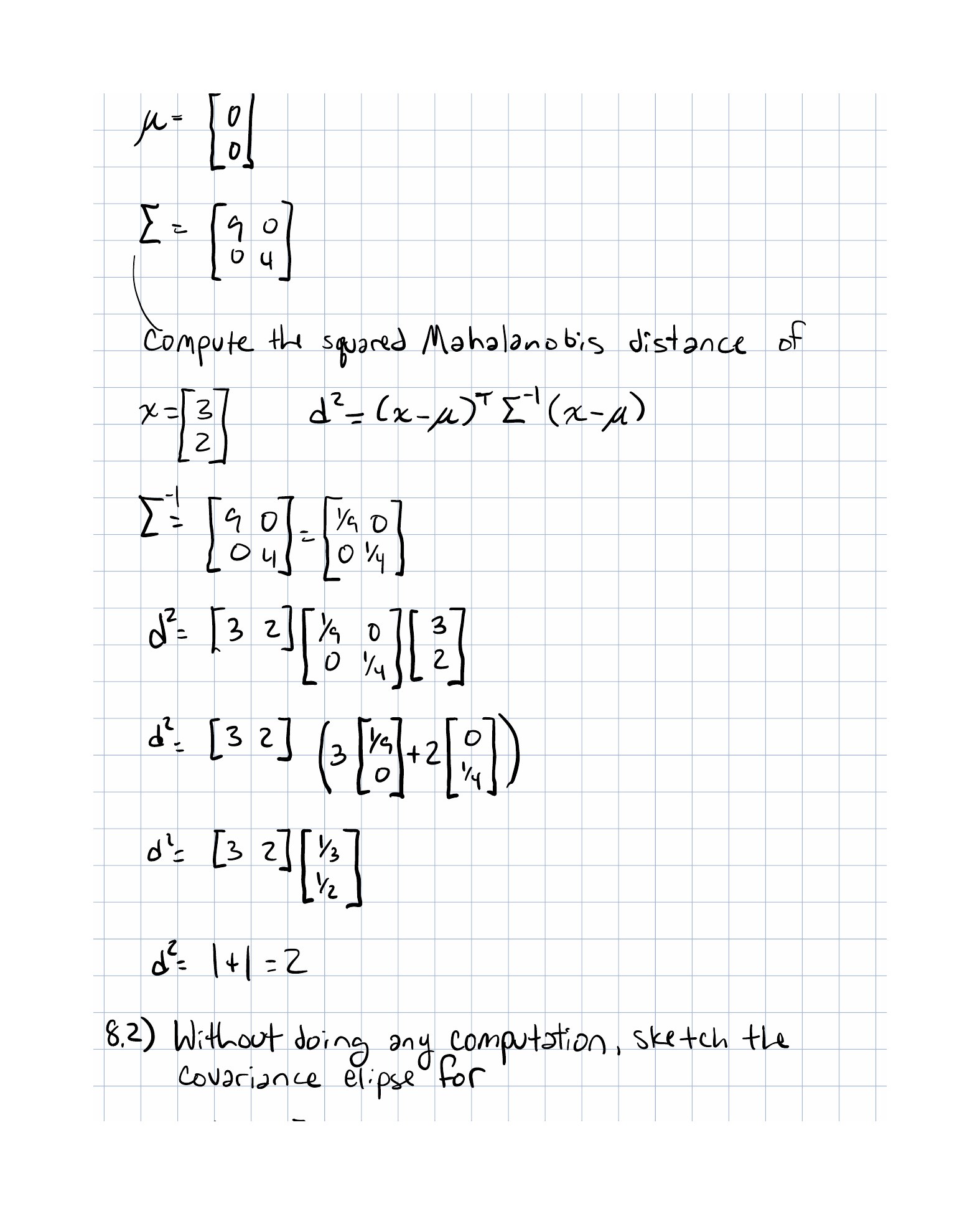
The squared Mahalanobis distance is
Core Ideas
Covariance turns circles into ellipses
In ordinary Euclidean geometry, points at fixed squared distance from the origin satisfy
That gives a circle in two dimensions or a sphere in higher dimensions.
When covariance enters, the relevant quadratic form becomes
Level sets of this expression are ellipses or ellipsoids. The covariance matrix stretches and rotates the geometry.
Why the inverse covariance appears
Large variance means motion in that direction is unsurprising. Small variance means motion in that direction is surprising.
So the distance metric should:
- penalize high-variance directions less;
- penalize low-variance directions more.
That is exactly what the inverse covariance does. If one direction has variance , the corresponding precision is , which makes movement in that direction contribute less to the distance.
Mahalanobis distance is Euclidean distance in whitened space
Whitening uses
Then
So the Mahalanobis distance is not a brand-new species of distance. It is ordinary Euclidean distance after the right change of coordinates.
The Gaussian density is the right exponential of distance
The one-dimensional Gaussian uses squared distance divided by variance:
The multivariate version replaces ordinary squared distance with squared Mahalanobis distance:
Nothing mystical happened. We took the one-dimensional idea and upgraded the geometry.
The determinant normalizes by volume
The determinant measures how covariance stretches volume.
If covariance spreads the distribution out across a larger ellipsoid, the peak density must be lower so the total probability still integrates to .
So the determinant is doing the same kind of job it always does in linear algebra: measuring how a transformation scales volume.
Eigenvectors and eigenvalues explain the shape
If
then the eigenvectors give the principal axes of the Gaussian ellipsoid. The eigenvalues give the variances along those axes.
The semi-axis lengths are proportional to
So large eigenvalues correspond to broad directions of uncertainty, while small eigenvalues correspond to narrow directions of confidence.
Worked Example
Let
Then
Now compute the squared Mahalanobis distance:
Interpretation:
- moving units in the first coordinate is exactly one standard deviation because ;
- moving units in the second coordinate is exactly one standard deviation because .
So this point sits one standard deviation away along each principal axis.
Why This Shows Up In ML
Gaussians show up all over machine learning because they are mathematically tractable and geometrically expressive.
Examples include:
- Gaussian noise models for regression;
- Gaussian priors in Bayesian methods;
- Kalman filters and state-space models;
- anomaly detection with Mahalanobis distance;
- latent-variable models such as variational autoencoders.
The broader lesson is that linear algebra is now describing uncertainty rather than only transformations.
Exercises
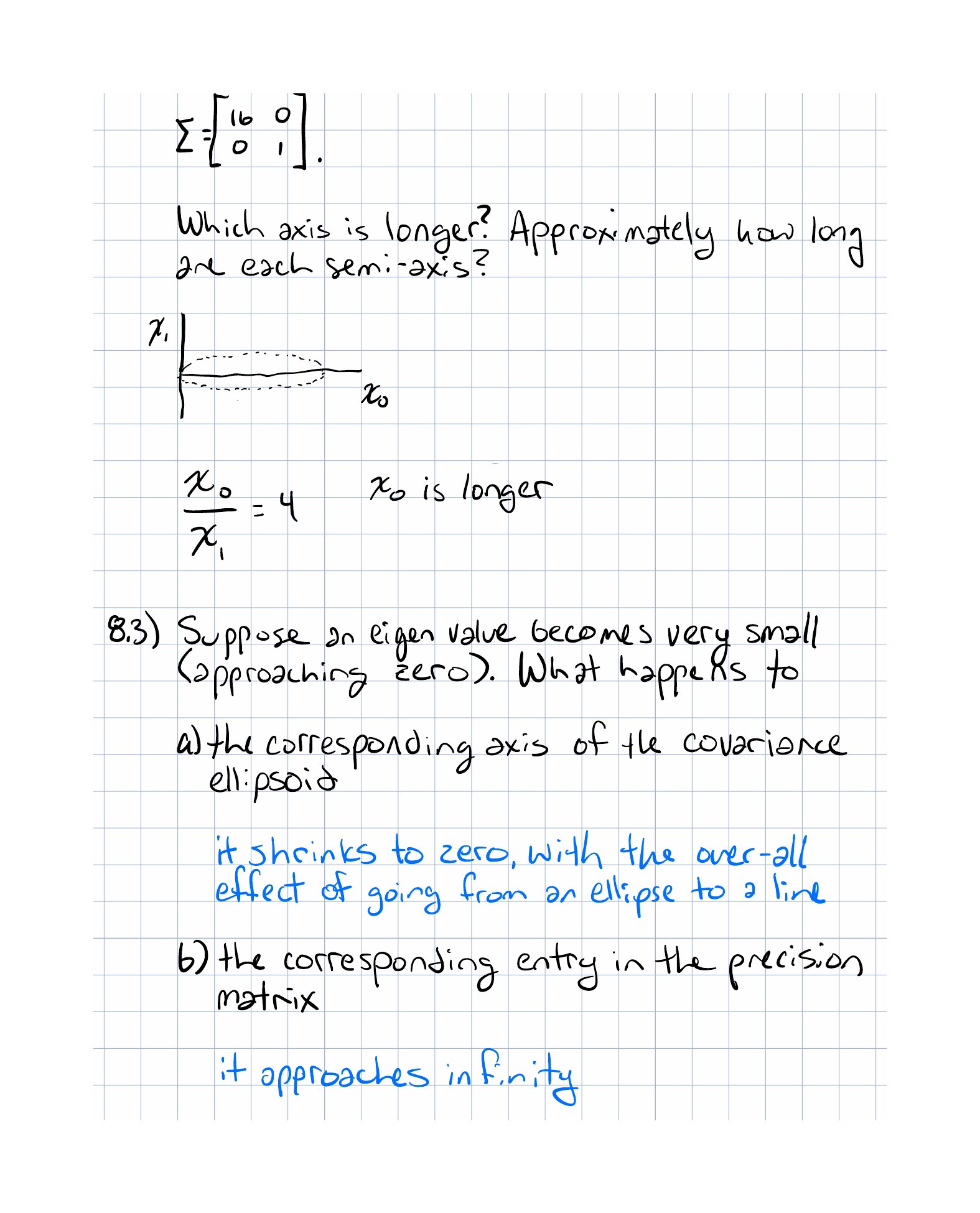
- For
sketch the covariance ellipse and label its semi-axis lengths.
- If an eigenvalue of becomes extremely small, what happens to:
- the corresponding axis of the ellipsoid;
- the corresponding precision;
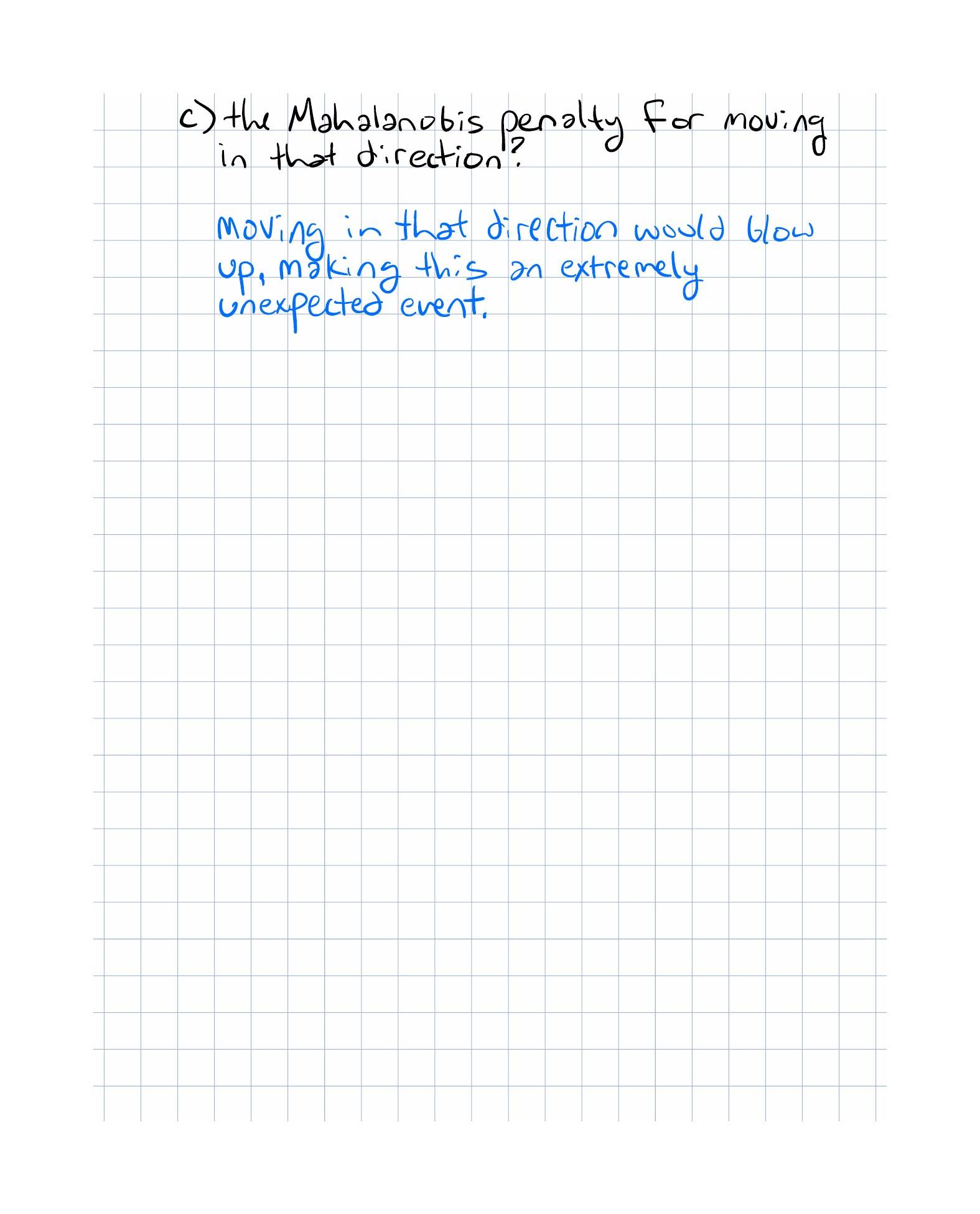
- the Mahalanobis penalty for moving in that direction?
-
Explain in words why the Gaussian formula uses in the exponent and in the normalization constant.
-
Why does whitening turn a multivariate Gaussian into a spherical one?
Implementation Exercise
Write a TypeScript function that evaluates the log density of a two-dimensional Gaussian.
Start with a diagonal covariance matrix so the inverse and determinant are easy to compute by hand. Then extend the function so it accepts:
- a mean vector;
- a covariance matrix;
- a point .
Keep the implementation explicit about each mathematical piece: centered vector, precision-weighted quadratic form, and determinant-based normalization.
Reflection Questions
- What feels more intuitive now: the formula for the Gaussian or the ellipse picture behind it?
- Why is the precision matrix a better name than “inverse covariance” once the geometry is clear?
- How does whitening simplify both the distance and the distribution?
- When you see a covariance matrix now, do you automatically picture an ellipsoid?
Completed Exercises
Handwritten work submitted after completing this lesson.