Lesson 16: Maximum Likelihood Estimation

Goal

Understand maximum likelihood estimation as a scoring rule for parameter choices: keep the data fixed, vary the parameter, and ask which value makes the observed data most plausible.

By the end of this lesson, you should be able to look at a simple dataset, write down its likelihood function, and explain why the best estimate is the parameter value that maximizes that function.

Motivation

Once we start using probabilistic models, a new question appears:

We know how to describe uncertainty.
We know how to write down distributions.
We know a model may contain unknown parameters.

How do we choose those parameters from real data?

That is what MLE answers. It is the bridge from “here is a statistical model” to “here is how we fit the model.”

A useful intuition is:

MLE treats each possible parameter value like a candidate explanation for the data, then scores those explanations by how well they predict what we actually saw.

This idea turns up everywhere in machine learning. Linear regression, logistic regression, Naive Bayes, Gaussian models, and many neural-network losses can all be understood as likelihood-based fitting.

Prerequisites

Lesson 13: Probability as Linear Algebra.
Lesson 15: Multivariate Gaussian.
Comfort with products of independent probabilities.
A rough sense that parameters describe the behavior of a model.

Notation / Symbol Table

Symbol	Plain-English name	Meaning
$\theta$	parameter	An unknown quantity that controls the model.
$D$	data	The observations we have already collected.
$P(D \mid \theta)$	probability of the data given theta	How probable the observed data would be if theta were the true parameter.
$L(\theta)$	likelihood	The same expression, but now treated as a function of theta.
$\ell(\theta)$	log-likelihood	$\log L(\theta)$ , used because it is easier to compute and optimize.
$\hat{\theta}$	estimate	The parameter value chosen by the estimation rule.
$k$	number of successes	How many times an event of interest occurred.
$n$	number of trials	Total number of observations in a repeated experiment.

The maximum likelihood estimate is written

\hat{\theta}_{MLE} = \arg\max_{\theta} L(\theta).

Read that as:

Choose the parameter value that gives the largest likelihood score.

Core Ideas

Likelihood Reuses Probability From A Different Viewpoint

Suppose a bag contains red and blue marbles, but we do not know the fraction of red marbles. Let

\theta = P(\text{Red}).

If someone tells us $\theta = 0.75$ , then

P(D \mid \theta)

is an ordinary probability statement:

If the red probability really were 0.75, how likely is this dataset?

Now flip the viewpoint. The dataset is already fixed. We observed it. What we do not know is $\theta$ .

Then the same expression becomes a score over parameter values:

L(\theta) = P(D \mid \theta).

The algebra did not change. The role of the symbols changed.

In probability, the parameter is fixed and the data could vary.
In likelihood, the data is fixed and the parameter varies.

That distinction is small on paper and enormous in practice.

Building A Likelihood Function

Suppose we observe

R R R B R

There are four reds and one blue. Under the parameter

\theta = P(R),

the likelihood is

L(\theta) = \theta^4 (1 - \theta).

Why?

Each red contributes a factor of $\theta$ .
Each blue contributes a factor of $1 - \theta$ .
Independent observations multiply.

This is the general pattern for many models:

Write down the probability of one observation under the parameter.
Assume independence when appropriate.
Multiply the per-example probabilities together.
Optimize the resulting likelihood.

The Best Estimate Is The Best Explanation Score

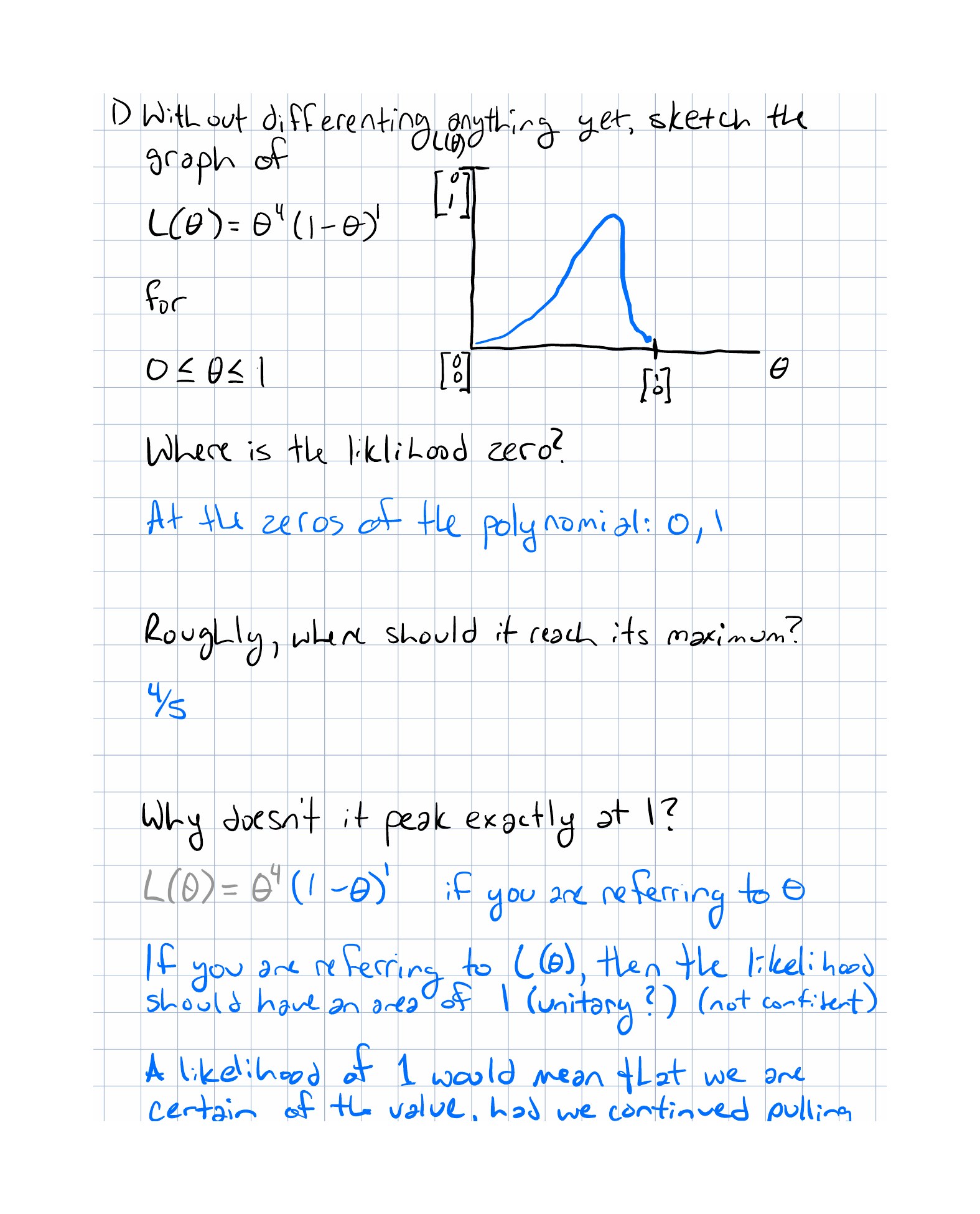
The likelihood for the marble example is zero at $\theta = 0$ and $\theta = 1$ .

$\theta = 0$ says red never happens, but we saw many reds.
$\theta = 1$ says blue never happens, but we saw one blue.

So the maximum must occur somewhere in between. Intuitively, the estimate should be close to the observed fraction of reds:

\frac{4}{5}.

That intuition generalizes. For repeated Bernoulli-style observations, the MLE often lands at the empirical frequency.

A Likelihood Is Not A Probability Distribution Over Parameters

This is the conceptual trap that catches almost everyone at first.

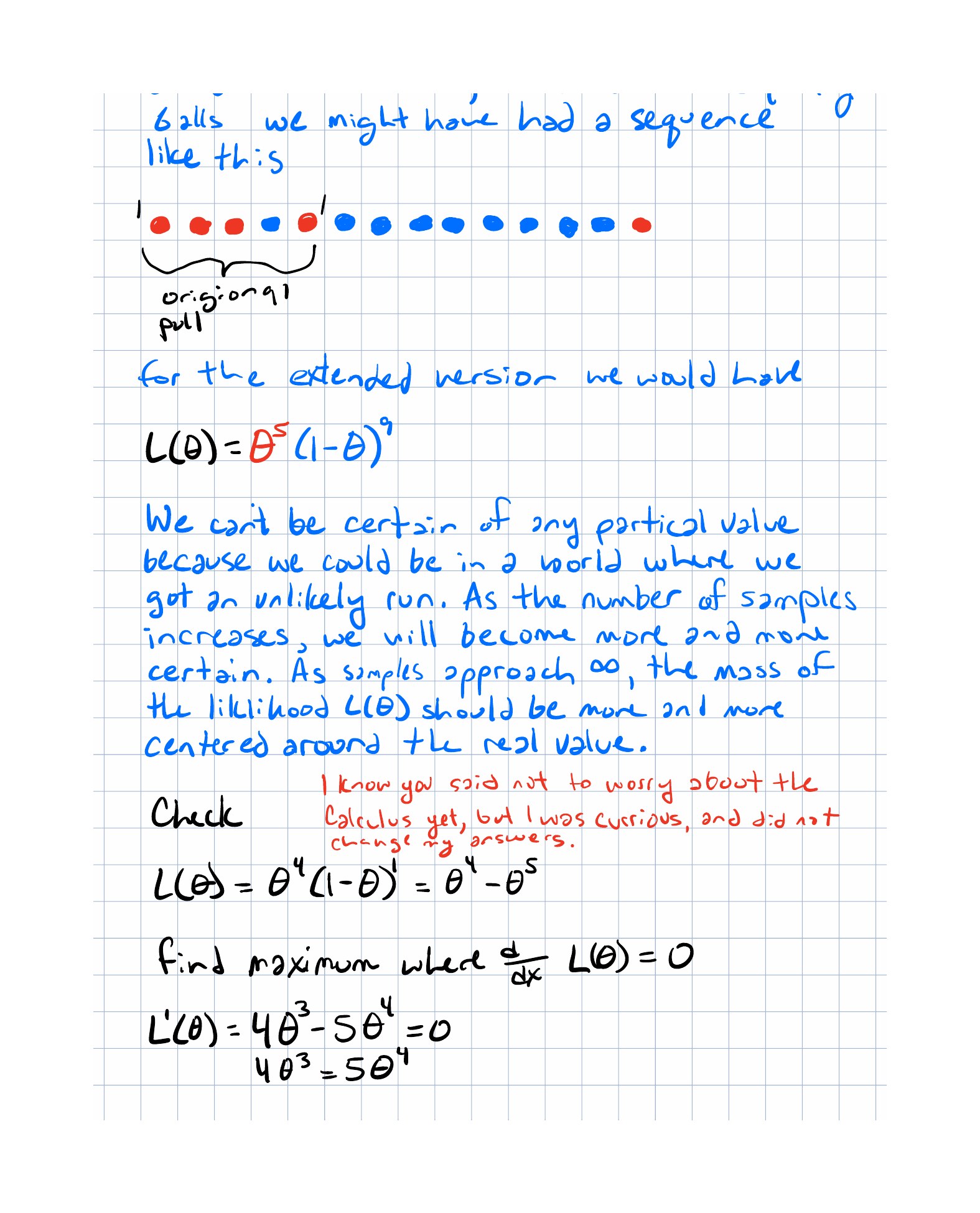
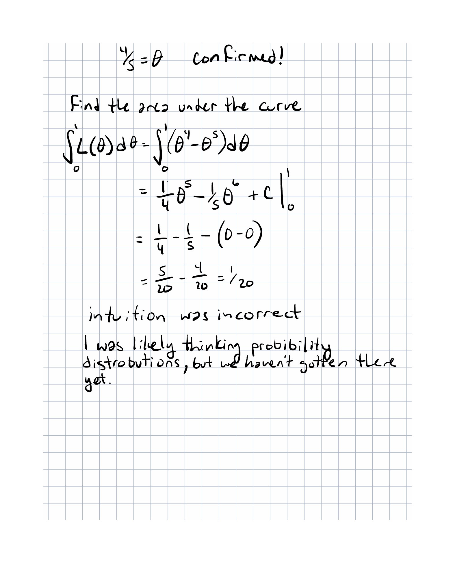
The function $L(\theta)$ is not required to integrate to 1 over $\theta$ . Its total area is not the point. A likelihood is a relative score, not a normalized belief distribution.

If we define

L'(\theta) = 10^9 L(\theta),

then every likelihood value becomes a billion times larger, but the maximizing parameter does not move.

That gives us a practical rule:

In maximum likelihood, only comparisons matter.

Absolute scale is arbitrary.

Why Log-Likelihood Takes Over

Large datasets make raw likelihoods awkward:

L(\theta) = \prod_{i=1}^{n} P(x_i \mid \theta).

Taking logs gives

\ell(\theta) = \log L(\theta) = \sum_{i=1}^{n} \log P(x_i \mid \theta).

This helps in two ways:

Products become sums.
Tiny probabilities stop underflowing as quickly.

Because the logarithm is strictly increasing, it preserves which parameter is best:

\arg\max_{\theta} L(\theta) = \arg\max_{\theta} \ell(\theta).

So we switch representations without changing the estimate.

Worked Example

Consider five coin flips with four heads and one tails. Let

\theta = P(H).

Then

L(\theta) = \theta^4 (1 - \theta).

We can reason about the shape before doing calculus:

$L(0) = 0$ because heads occurred and $\theta = 0$ says heads are impossible.
$L(1) = 0$ because tails occurred and $\theta = 1$ says tails are impossible.
The curve should rise toward values near 0.8 because most observations were heads.
It should not peak at 1 because that would completely fail to explain the tails observation.

If we now take logs,

\ell(\theta) = 4 \log \theta + \log(1 - \theta),

which is much easier to differentiate than the original product form.

Even before solving formally, the lesson is already visible:

The best-fitting parameter balances the evidence from all observations, and the log turns that balance into simple addition.

Why This Shows Up In ML

Machine learning models usually contain parameters we do not know in advance:

regression coefficients,
class probabilities,
Gaussian means and variances,
neural-network weights.

Likelihood gives a general recipe for fitting them:

Write down a probability model for the data.
Treat the observed dataset as fixed.
Score each parameter value by how plausible it makes the data.
Choose the maximizing parameter, usually through the log-likelihood.

This is why MLE is so central. It turns modeling assumptions into an optimization problem.

It also explains why later lessons talk so much about loss functions. Once we take logs and change signs, many familiar ML objectives are just transformed likelihoods.

Exercises

Use a simple Bernoulli model and answer the following in words before computing anything:

If you observe H H H T H, where should the MLE for $\theta$ be roughly located?
Why does the likelihood become zero at $\theta = 0$ and $\theta = 1$ ?
Why does multiplying a likelihood by 50 not change the estimate?
What is the difference between “probability of the data given theta” and “likelihood of theta given the data”?

Then write the likelihood for:

H, T, H, H, T, H.

Implementation Exercise

Write a TypeScript helper for Bernoulli likelihoods:

type BernoulliSample = 0 | 1;

const likelihood = (theta: number, samples: BernoulliSample[]): number =>
  samples.reduce(
    (product, sample) => product * (sample === 1 ? theta : 1 - theta),
    1,
  );

Then extend it to compute the log-likelihood directly so you can compare:

raw likelihood values,
log-likelihood values,
the grid point where each is maximized.

Use a small grid such as 0.01, 0.02, ..., 0.99 and confirm that both methods pick the same best parameter.

Reflection Questions

Which part of MLE felt like a viewpoint change rather than a new formula?
Why is “likelihood is not a probability distribution over parameters” such an important correction?
When do products become painful enough that logs feel necessary rather than optional?
In the marble or coin example, what information is being discarded when we report only a single best estimate?

Completed Exercises

Handwritten work submitted after completing this lesson.