Lesson 17: Loss Functions | Mathematics of AI

Goal

Understand why machine learning usually talks about minimizing a loss instead of maximizing a likelihood, and why these are often the same optimization problem written in different forms.

By the end of this lesson, you should be able to explain why least squares comes from a Gaussian noise assumption rather than appearing as an arbitrary design choice.

Motivation

MLE gave us a clean principle:

Choose the parameter values that make the observed data most likely.

But machine learning code, papers, and libraries usually do not say “maximize likelihood.” They say things like:

minimize loss,
minimize error,
optimize objective,
reduce training cost.

Why the change in language?

Because optimization systems like minimization. Also, once we take logs and drop constants, the resulting expressions are easier to compute, easier to differentiate, and easier to recognize across models.

This lesson is the moment where statistics starts looking like optimization.

Prerequisites

Lesson 15: Multivariate Gaussian.
Lesson 16: Maximum Likelihood Estimation.
Comfort with logarithms, especially that $\log(ab) = \log a + \log b$ .
Basic familiarity with model predictions and residuals.

Notation / Symbol Table

Symbol	Plain-English name	Meaning
$D$	dataset	The full collection of observed examples.
$\theta$	parameters	The values the model can change during fitting.
$L(\theta)$	likelihood	Probability or density of the data under the model.
$\ell(\theta)$	log-likelihood	$\log L(\theta)$ .
$-\ell(\theta)$	negative log-likelihood	A minimization version of the same fitting objective.
$x_i$	input	Features for example $i$ .
$y_i$	target	Observed output for example $i$ .
$f_{\theta}(x_i)$	prediction	Model output for input $x_i$ .
$\epsilon_i$	noise	Difference between observation and prediction.
$\sigma^2$	noise variance	Spread of the Gaussian error model.

The core transformation is

\hat{\theta} = \arg\max_{\theta} L(\theta) = \arg\max_{\theta} \ell(\theta) = \arg\min_{\theta} \bigl(-\ell(\theta)\bigr).

Core Ideas

Log-Likelihood Keeps The Same Best Parameters

For independent observations,

L(\theta) = \prod_i P(x_i \mid \theta).

Taking logs turns this into

\ell(\theta) = \sum_i \log P(x_i \mid \theta).

This does not change the maximizing parameter because the logarithm preserves ordering.

That means the log-likelihood is not a new objective. It is a friendlier encoding of the old one.

Negative Log-Likelihood Turns Maximization Into Minimization

Many optimization tools are built around minimization. So after taking logs, we flip the sign:

\text{Loss}(\theta) = -\ell(\theta).

Now the question becomes:

Which parameters make the penalty as small as possible?

This is just a convention, but it is a powerful one. It makes very different models look structurally similar.

A Loss Function Often Falls Out Of A Probability Model

This is the key lesson:

Many standard loss functions are negative log-likelihoods.

Examples:

Gaussian observation model -> squared-error style loss.
Bernoulli observation model -> cross-entropy style loss.
Laplace observation model -> absolute-error style loss.

So a loss function is often not something we invent from taste. It is something implied by the distribution we chose for the data.

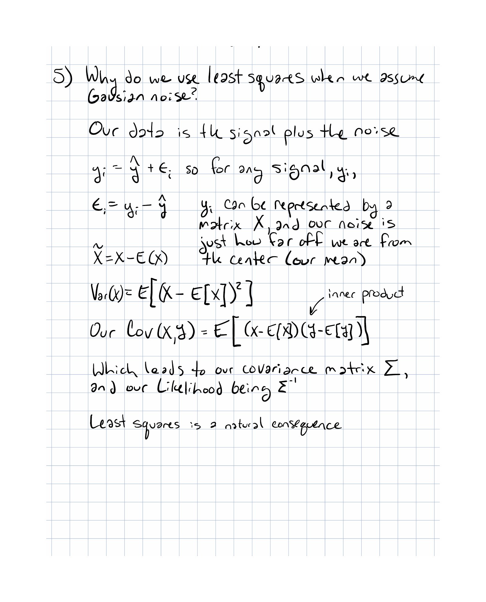
Gaussian Noise Produces Squared Error

Suppose the model is

y_i = f_{\theta}(x_i) + \epsilon_i

with

\epsilon_i \sim \mathcal{N}(0, \sigma^2).

This says:

Observed value = model prediction + random Gaussian noise.

Under this assumption, the conditional density of $y_i$ is

P(y_i \mid x_i, \theta) = \frac{1}{\sqrt{2\pi \sigma^2}} \exp\left( -\frac{(y_i - f_{\theta}(x_i))^2}{2\sigma^2} \right).

Taking logs gives

\log P(y_i \mid x_i, \theta) = -\frac{(y_i - f_{\theta}(x_i))^2}{2\sigma^2} + \text{constant}.

Summing over the dataset and negating yields

-\ell(\theta) = \frac{1}{2\sigma^2} \sum_i (y_i - f_{\theta}(x_i))^2 + \text{constant}.

Everything except the squared residual term is constant with respect to $\theta$ . So minimizing the negative log-likelihood is equivalent to minimizing

\sum_i (y_i - f_{\theta}(x_i))^2.

That is the least-squares objective.

Constants And Positive Rescaling Need Different Attention

Two common transformations behave differently:

Add a constant:
$J'(\theta) = J(\theta) + 5000$
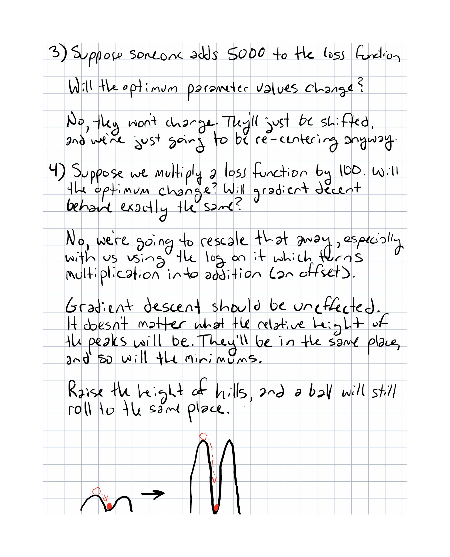
The optimum does not change, and the gradients do not change either.
Multiply by a positive constant:
$J'(\theta) = 100 J(\theta)$
The optimum still does not change, but the gradients become 100 times larger.

That second point matters once we start using gradient descent. The best parameter can stay the same while the optimization path changes a lot.

Worked Example

Assume a one-parameter regression model predicts

\hat{y}_i = f_{\theta}(x_i)

and the observed targets satisfy

y_i = \hat{y}_i + \epsilon_i, \qquad \epsilon_i \sim \mathcal{N}(0, \sigma^2).

For one example, the density is

P(y_i \mid x_i, \theta) = \frac{1}{\sqrt{2\pi \sigma^2}} \exp\left( -\frac{(y_i - \hat{y}_i)^2}{2\sigma^2} \right).

Now apply the sequence slowly:

Multiply these terms across independent examples to get the likelihood.
Take logs so the product becomes a sum.
Negate so we can minimize instead of maximize.
Drop constants that do not depend on $\theta$ .

What survives is the sum of squared residuals.

That is the whole punchline:

Squared-error loss is the optimization face of a Gaussian probabilistic model.

Why This Shows Up In ML

When ML practitioners choose a loss, they are often making a statement about the data-generating process.

Squared error says large deviations become exponentially less plausible in a Gaussian way.
Cross-entropy says the target behaves like a Bernoulli or categorical draw.
Absolute error says errors are better modeled by a Laplace-style distribution.

This connection is valuable because it lets us reason in both directions:

Start from a probabilistic assumption and derive the loss.
Inspect a loss and ask what statistical assumptions it implies.

That is one of the big organizing ideas in statistical machine learning.

Exercises

Answer these in words first, then with formulas:

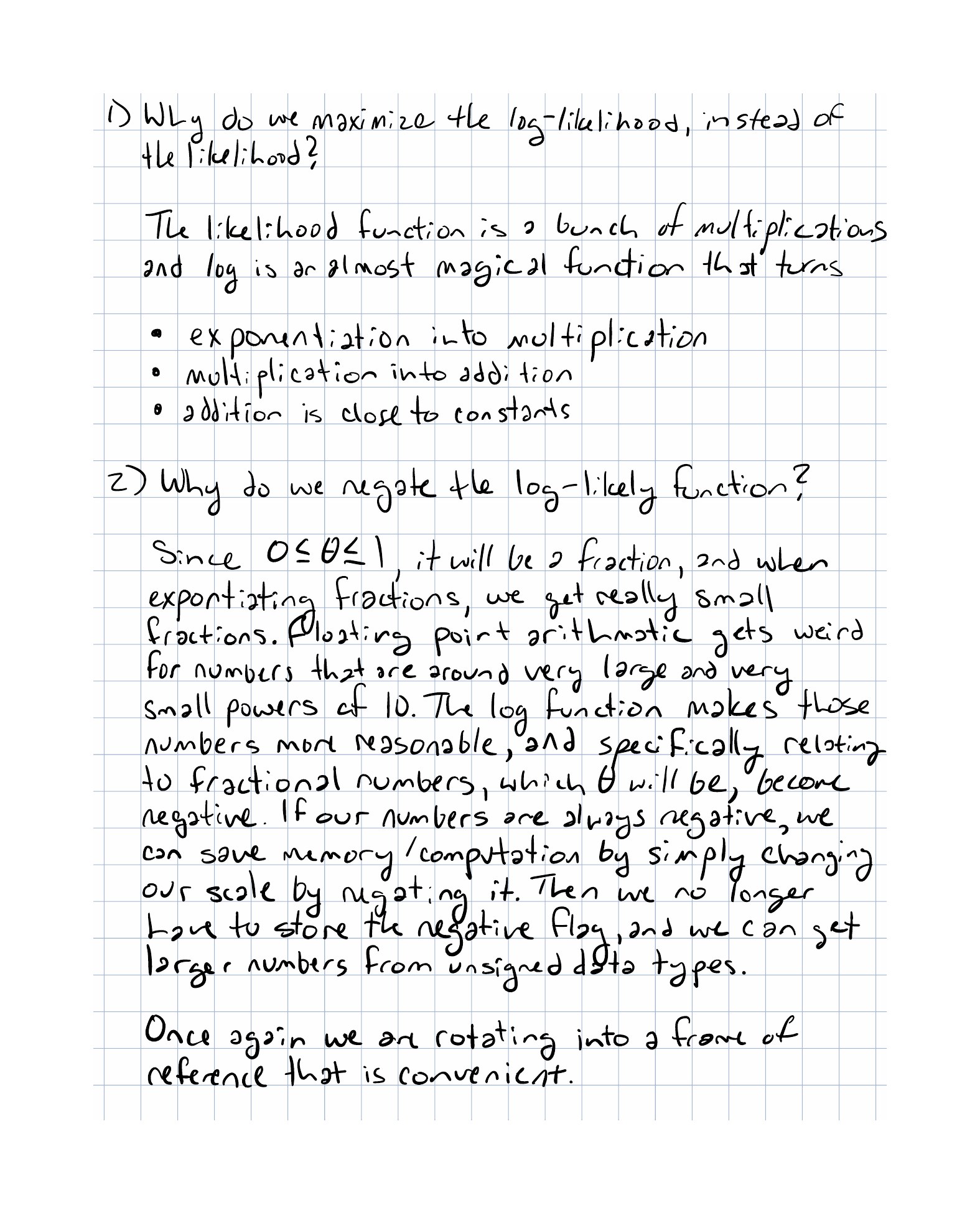
Why does maximizing log-likelihood pick the same optimum as maximizing likelihood?
Why do we introduce the negative sign after taking logs?
If we add +5000 to a loss, what changes and what stays the same?
If we multiply a loss by 100, what stays the same and what changes once gradient descent enters the picture?
In one paragraph, explain why least squares emerges naturally from a Gaussian noise assumption.

Implementation Exercise

Write a TypeScript function that computes a Gaussian negative log-likelihood for a fixed variance:

type Example = { x: number; y: number };

const gaussianNll = (
  examples: Example[],
  predict: (x: number, theta: number) => number,
  theta: number,
  sigma2: number,
): number =>
  examples.reduce((total, { x, y }) => {
    const residual = y - predict(x, theta);
    return total + residual ** 2 / (2 * sigma2);
  }, 0);

Then compare its minimizer against the minimizer of plain squared error on a small grid of parameter values. They should occur at the same place when sigma2 is fixed.

Reflection Questions

Which feels more fundamental to you now: the loss or the probability model behind it?
Why is dropping constants mathematically legitimate but multiplying by a positive constant operationally meaningful for optimization?
When you see a named loss in an ML paper, do you now want to ask what likelihood produced it?
Which symbols in the Gaussian derivation should become part of the course-wide notation reference?

Completed Exercises

Handwritten work submitted after completing this lesson.