Lesson 18: MAP Estimation | Mathematics of AI

Goal

Understand maximum a posteriori estimation as the version of parameter fitting that keeps the data term from MLE but adds a prior preference over parameter values.

By the end of this lesson, you should be able to explain why Gaussian priors lead to L2 regularization and why MAP and MLE become closer as the dataset gets larger.

Motivation

MLE asks a clean question:

Which parameter makes the observed data most likely?

But sometimes that question feels incomplete. If two noisy points suggest a line with slope 500, MLE may happily choose it if it fits the observations best.

Human intuition pushes back:

some parameter values feel too extreme,
some models feel too brittle,
some explanations feel implausible before we even look at this particular dataset.

MAP is the formal version of that pushback. It lets us say:

Fit the data well, but do not ignore what we already considered plausible.

Prerequisites

Lesson 16: Maximum Likelihood Estimation.
Lesson 17: Loss Functions.
Familiarity with Bayes’ rule in the abstract.
Comfort reading Gaussian densities and squared-error objectives.

Notation / Symbol Table

Symbol	Plain-English name	Meaning
$D$	data	The observations already collected.
$\theta$	parameter	The unknown quantity or vector we want to estimate.
$P(D \mid \theta)$	likelihood	How well theta explains the observed data.
$P(\theta)$	prior	How plausible theta seemed before seeing the data.
$P(\theta \mid D)$	posterior	Updated plausibility after seeing the data.
$P(D)$	evidence	Normalization constant that does not depend on theta.
$\hat{\theta}_{MAP}$	MAP estimate	The parameter value with the highest posterior probability or density.
$\tau^2$	prior variance	Spread of a Gaussian prior over parameters.
$\lambda$	regularization strength	A positive constant that scales the penalty term.

The MAP rule is

\hat{\theta}_{MAP} = \arg\max_{\theta} P(\theta \mid D).

Using Bayes’ rule,

\hat{\theta}_{MAP} = \arg\max_{\theta} P(D \mid \theta) P(\theta),

because $P(D)$ is constant with respect to $\theta$ .

Core Ideas

MAP Adds A Prior To The MLE Story

MLE only scores data fit:

\hat{\theta}_{MLE} = \arg\max_{\theta} P(D \mid \theta).

MAP scores both data fit and prior plausibility:

\hat{\theta}_{MAP} = \arg\max_{\theta} P(D \mid \theta) P(\theta).

So the two methods differ by one extra ingredient:

MLE asks which parameter best explains this dataset.
MAP asks which parameter best explains this dataset after accounting for prior beliefs.

Bayes’ Rule Separates The Roles Cleanly

Bayes’ rule for parameter estimation is

P(\theta \mid D) = \frac{P(D \mid \theta) P(\theta)}{P(D)}.

Each term has a distinct job:

likelihood: evidence from the data,
prior: what we believed before,
posterior: updated belief,
evidence: normalization.

For optimization, the evidence is ignorable because it does not depend on $\theta$ .

Taking Logs Turns The Product Into A Sum

Optimizing the posterior directly can be awkward, so we take logs:

\log P(\theta \mid D) = \log P(D \mid \theta) + \log P(\theta) - \log P(D).

Ignoring the last term during optimization leaves two forces:

a data-fit term,
a prior term.

That is the shape regularized ML objectives often take.

Gaussian Prior -> Quadratic Penalty

Suppose we believe parameters are usually near zero:

\theta \sim \mathcal{N}(0, \tau^2).

Then the prior density is

P(\theta) = \frac{1}{\sqrt{2\pi \tau^2}} \exp\left( -\frac{\theta^2}{2\tau^2} \right).

Taking logs and ignoring constants gives

\log P(\theta) = -\frac{\theta^2}{2\tau^2} + \text{constant}.

Negating that contribution produces a quadratic penalty:

\frac{\theta^2}{2\tau^2}.

For a parameter vector, this becomes a scaled squared L2 norm:

\lambda \lVert \theta \rVert_2^2.

This is the mathematical core of L2 regularization.

Regularization Is A Prior In Disguise

This is the big insight:

A Gaussian likelihood gave us squared-error data fit. A Gaussian prior gives us an L2 penalty.

Put them together and MAP optimization becomes

\text{data-fit term} + \text{regularization term}.

So regularization is not just a trick for making models behave. It is one way of encoding prior beliefs about reasonable parameter size.

The Prior Matters Most When Data Is Scarce

If the dataset is tiny, the likelihood is broad and many parameter values may fit reasonably well. Then the prior can noticeably shift the estimate.

If the dataset is enormous, the likelihood becomes sharply concentrated and the prior usually matters much less.

That gives a good intuition for the MLE versus MAP gap:

small data -> prior matters more,
large data -> data dominates.

Worked Example

Suppose a simple regression problem has only a few noisy observations, and an unconstrained fit suggests a very large slope.

Under MLE, we would choose the slope that best fits those observations.

Under MAP, we multiply the likelihood by a prior that says very large slopes are less plausible:

P(\theta \mid D) \propto P(D \mid \theta) P(\theta).

If the prior is Gaussian around zero, then very large values of $\theta$ receive an exponential penalty. After taking logs, this becomes a quadratic cost on parameter size.

The result is not that the model refuses to learn large weights. The result is subtler:

Large weights are allowed, but they must earn their way by improving data fit enough to overcome the prior penalty.

That is exactly the behavior people describe informally when they talk about regularization discouraging overly complex models.

Why This Shows Up In ML

Many ML training objectives have this form:

\text{loss} = \text{fit to data} + \text{penalty on parameters}.

MAP explains where that structure comes from.

Data-fit term -> negative log-likelihood.
Penalty term -> negative log-prior.

This perspective helps unify several ideas:

L2 regularization corresponds to a Gaussian prior.
L1 regularization corresponds to a Laplace prior.
Stronger regularization means a stronger preference for certain parameter values before seeing the data.

So when someone tunes regularization, they are also tuning an implicit prior belief.

Exercises

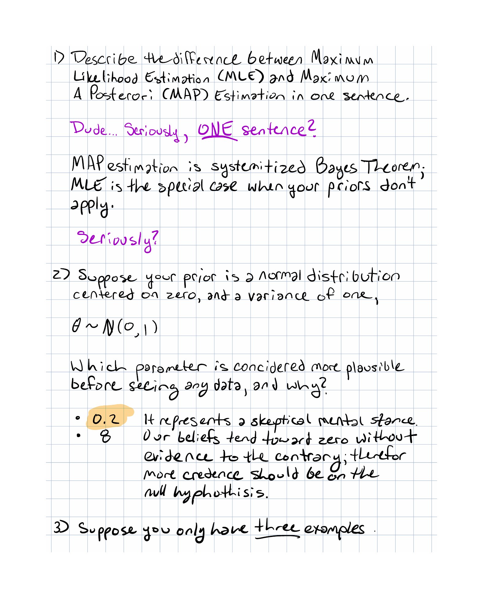
In one sentence, describe the difference between MLE and MAP.
Suppose the prior is $\theta \sim \mathcal{N}(0, 1)$ . Which is more plausible before seeing data: $\theta = 0.2$ or $\theta = 8$ ? Why?
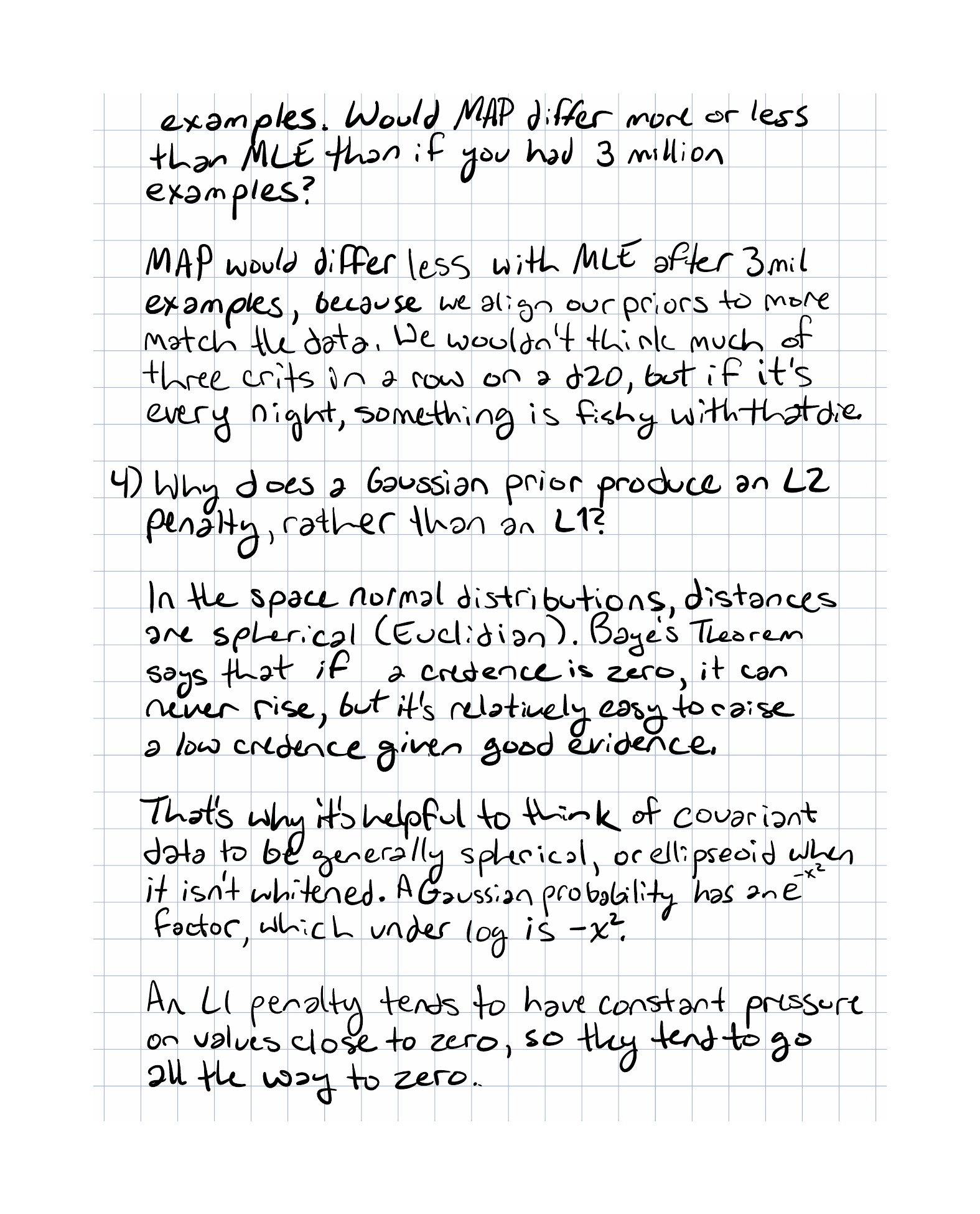
Why should MAP usually differ more from MLE with 3 examples than with 3 million examples?
Why does a Gaussian prior create an L2-style penalty instead of an L1-style penalty?
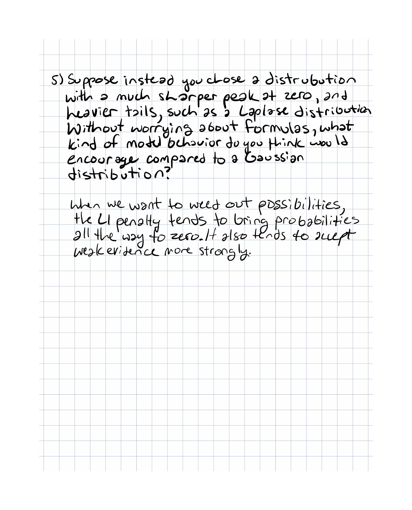
Without deriving anything, predict what kind of parameter behavior a Laplace prior would encourage relative to a Gaussian prior.

Implementation Exercise

Implement a regularized least-squares objective in TypeScript:

type Example = { x: number; y: number };

const objective = (
  examples: Example[],
  predict: (x: number, theta: number[]) => number,
  theta: number[],
  lambda: number,
): number =>
  examples.reduce((total, { x, y }) => {
    const residual = y - predict(x, theta);
    return total + residual ** 2;
  }, 0) + lambda * theta.reduce((total, value) => total + value ** 2, 0);

Then vary lambda and inspect how the minimizing parameter vector changes. Describe what happens to the magnitude of the learned weights as the prior gets stronger.

Reflection Questions

Did MAP feel like “new math” or like “MLE plus one more idea”?
What is the smallest algebraic fact that forces a Gaussian prior to become an L2 penalty?
When would you want a strong prior, and when would you want the data to speak more freely?
Which part of regularization now feels more principled than it did before this lesson?

Completed Exercises

Handwritten work submitted after completing this lesson.