Goal
Understand the conceptual shift from point estimation to Bayesian estimation: instead of asking for one best parameter, we keep a full probability distribution over plausible parameter values.
By the end of this lesson, you should be able to explain what extra information the posterior keeps that MLE and MAP throw away.
Motivation
MLE and MAP both end by reporting one parameter value:
- MLE gives the best likelihood explanation.
- MAP gives the best posterior explanation.
But sometimes one number is not enough.
Two parameter values might both be plausible. Or one estimate might be sharp and confident while another is vague and uncertain. A single winner cannot show that difference.
Bayesian estimation keeps the entire distribution:
Not just which parameter is best, but how plausible each parameter value is relative to the others.
That extra structure is the main reason Bayesian methods are so expressive.
Prerequisites
- Lesson 18: MAP Estimation.
- A working understanding of Bayes’ rule.
- Comfort thinking of a parameter as something unknown rather than fixed and fully known.
Notation / Symbol Table
| Symbol | Plain-English name | Meaning |
|---|---|---|
| parameter | The unknown quantity we want to learn about. | |
| data | The observed evidence. | |
| prior | Belief distribution before seeing the data. | |
| likelihood | How compatible the data is with each parameter value. | |
| posterior | Updated belief after incorporating the data. | |
| evidence | Normalizing constant that makes the posterior integrate to 1. |
Bayes’ rule for parameter estimation is
Core Ideas
Bayesian Estimation Keeps Uncertainty Explicit
Suppose we are estimating a coin’s bias .
Point estimation says something like:
Bayesian estimation says:
I do not know the true value exactly. I have a distribution over plausible values.
That distribution might be:
- narrow and sharply peaked,
- broad and uncertain,
- skewed toward one side,
- even multi-modal in more complex settings.
The posterior is an object that carries all of that information.
Prior, Likelihood, Posterior, Evidence
Each piece of Bayes’ rule answers a separate question:
- Prior : What seemed plausible before this dataset?
- Likelihood : Which parameter values would predict the observations well?
- Posterior : What seems plausible after combining prior and data?
- Evidence : What constant is needed so the posterior becomes a valid probability distribution?
The evidence is often the hardest term to feel intuitively. It is not an extra opinion about theta. It is the normalization step that turns an unscaled score into a proper distribution.
The Evidence Normalizes The Posterior
The denominator is
This expression sums up all the ways the model could have explained the observed data.
For point estimation tasks like MAP, we often ignore it because it does not change which theta is largest.
For full Bayesian estimation, we keep caring about it because we want the posterior to be a real probability distribution whose total mass is 1.
MAP Is One Summary Of The Posterior, Not The Posterior Itself
MAP picks the highest point of the posterior:
That can be useful, but it compresses the distribution down to one number.
What disappears when we do that?
- uncertainty width,
- asymmetry,
- nearby alternative hypotheses,
- confidence about how strongly one value beats another.
The posterior keeps all of that.
Width Matters
Imagine two posterior distributions with the same peak location:
- one is narrow and tall,
- one is wide and flat.
If we only report the mode, they look identical. But they mean very different things.
The narrow posterior says:
We have strong evidence concentrated near one parameter region.
The wide posterior says:
Many parameter values still fit reasonably well.
This is why Bayesian estimation is especially useful when we care about confidence, uncertainty, and downstream decisions.
Worked Example
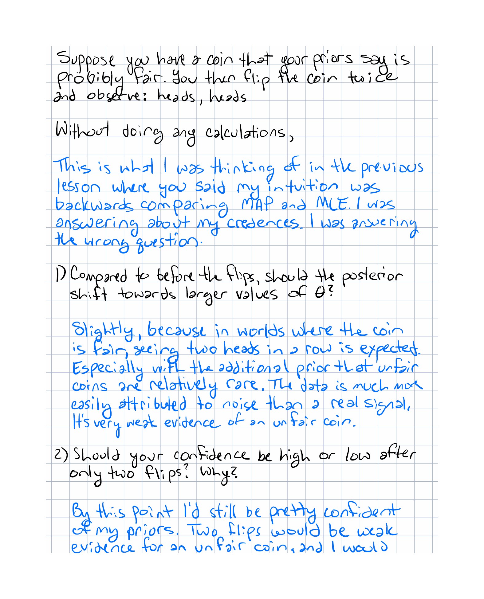
Suppose your prior for a coin is centered near fairness, and then you observe two heads in two flips.
A Bayesian update should do two things at once:
- Shift probability mass toward larger values of because heads are easier to explain when is larger.
- Keep the posterior fairly broad because two flips are not much evidence.
So the correct story is not “the coin bias is now 0.8” or any other single number. The correct story is:
The posterior moved to the right, but it is still wide.
That sentence carries both direction and uncertainty, which is exactly what Bayesian estimation is trying to preserve.
Why This Shows Up In ML
Machine learning often has to make decisions under uncertainty:
- Which parameters are plausible?
- How certain are we about them?
- How much should a new observation change our beliefs?
- How risky is a confident-looking prediction when the model is still uncertain?
Point estimates hide some of that information. Posterior distributions expose it.
Even when large-scale ML systems use approximations instead of exact Bayesian inference, the Bayesian picture still shapes the goals:
- quantify uncertainty,
- update with evidence,
- avoid pretending one point estimate tells the whole story.
Exercises
- In your own words, what extra information does the posterior contain that MAP does not?
- If you observe two heads in two flips, should the posterior move toward larger or smaller ? Should it become narrow or remain broad?
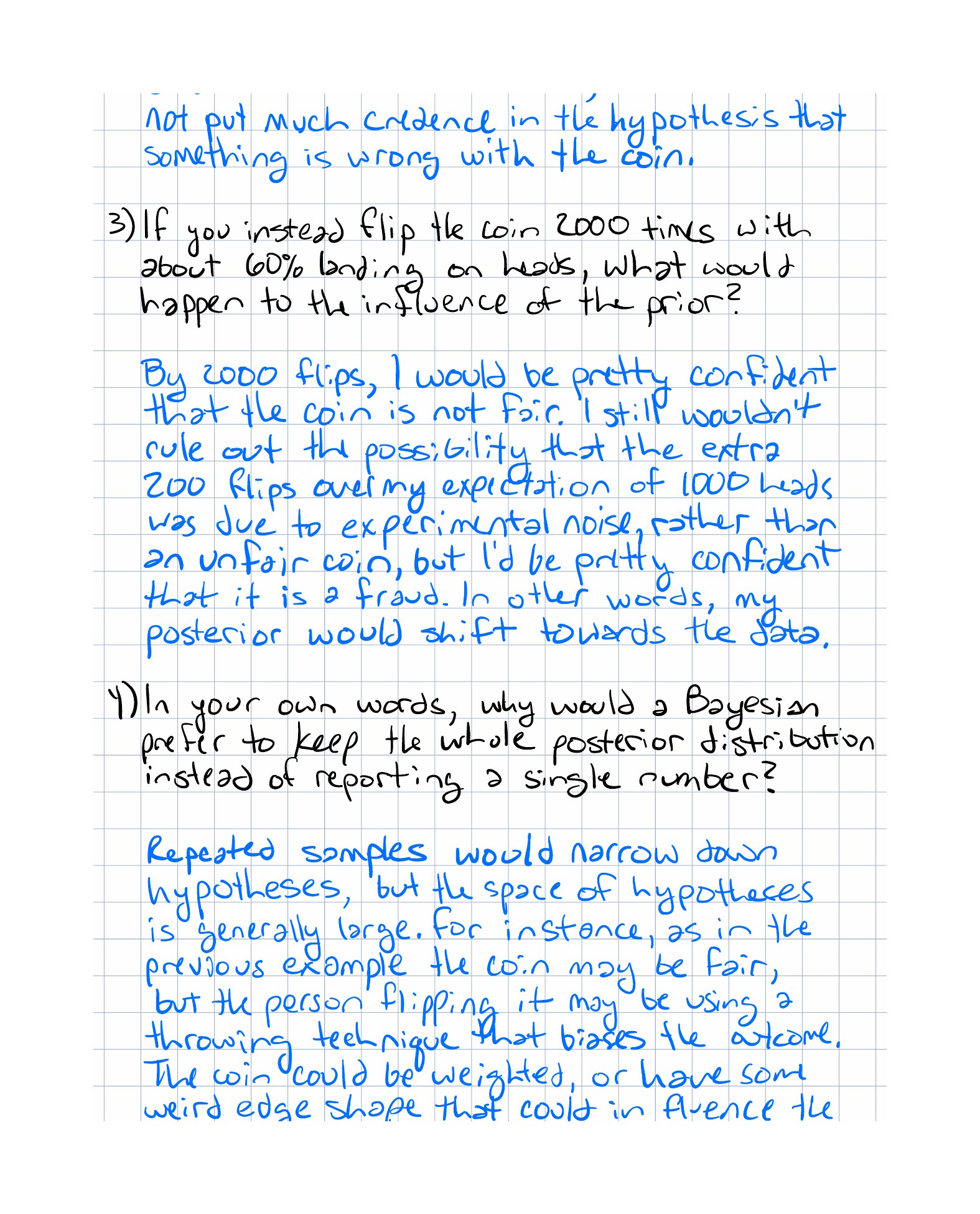
- Why does the prior matter less after 2,000 observations than after 2 observations?
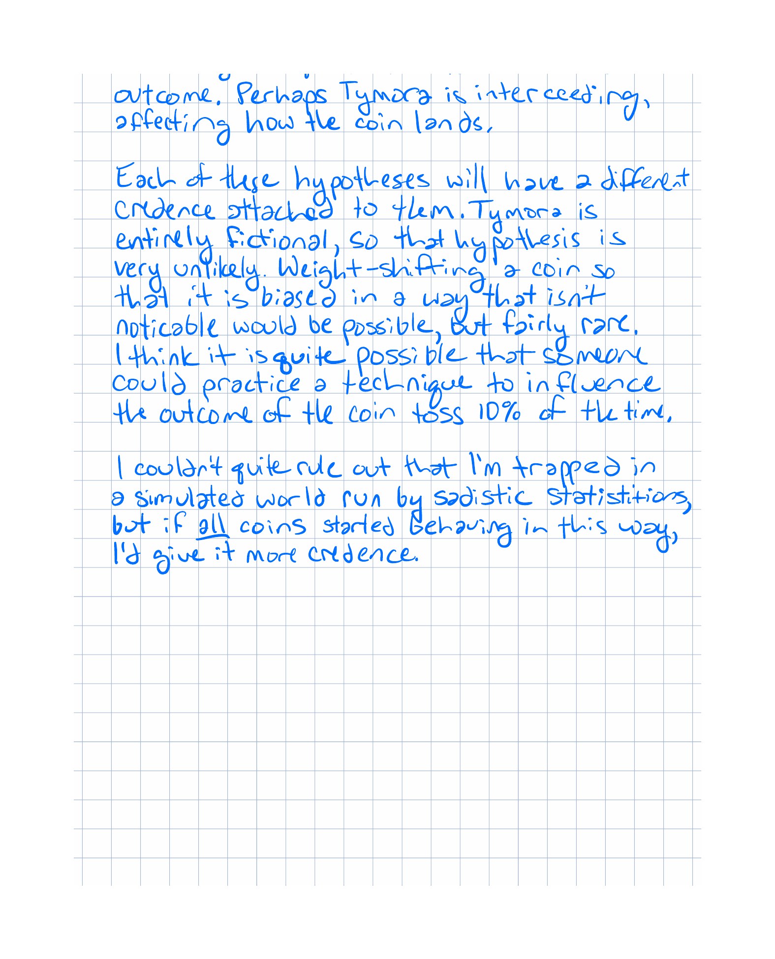
- Why would a Bayesian prefer to keep the whole posterior instead of reporting only the most likely parameter?
Implementation Exercise
Represent a discrete prior over coin-bias hypotheses in TypeScript:
type Hypothesis = {
  theta: number;
  prior: number;
};
Create a function that multiplies each prior weight by the Bernoulli likelihood of an observed flip, then normalizes the result to produce a posterior distribution over the finite hypothesis set.
Run it for a few hypotheses such as 0.3, 0.5, 0.7, and 0.9, and compare the posterior after:
- no flips,
- two heads,
- two hundred flips with about 60% heads.
Describe how the distribution’s width changes.
Reflection Questions
- What does it mean, emotionally and mathematically, to admit uncertainty about the parameter itself?
- When do you think a single point estimate is enough, and when is it hiding something important?
- Which piece of Bayes’ rule now feels most intuitive, and which still feels most mechanical?
- Did the posterior-width idea change how you think about “confidence” in a model?
Completed Exercises
Handwritten work submitted after completing this lesson.