Goal
Understand Bayesian updating as an actual step-by-step computation: score each hypothesis by prior times likelihood, normalize, and reuse the result as the next prior.
By the end of this lesson, you should be able to carry out a small discrete posterior update by hand and explain why repeated small updates are such a natural computational pattern.
Motivation
Lesson 19 introduced the posterior as a full distribution over parameters. This lesson makes that idea operational.
The main question is:
When a new observation arrives, how exactly do beliefs change?
The answer is simple enough to compute by hand:
- Start with prior probabilities.
- Multiply each one by how well it predicted the observation.
- Normalize so the probabilities sum to 1.
- Treat the result as the new prior for the next observation.
That loop is one of the cleanest expressions of learning from evidence anywhere in mathematics.
Prerequisites
- Lesson 19: Bayesian Estimation Introduction.
- Bayes’ rule in symbolic form.
- Comfort with small probability tables and normalization.
Notation / Symbol Table
| Symbol | Plain-English name | Meaning |
|---|---|---|
| hypothesis parameter | One candidate value of the unknown parameter. | |
| prior | Probability assigned to that hypothesis before the new observation. | |
| observation | A heads result in the coin example. | |
| likelihood | Probability that this hypothesis would produce heads. | |
| posterior | Probability of the hypothesis after seeing heads. | |
| proportional to | Equal up to a normalization constant. |
For one update,
Normalization then turns the proportional scores into a valid probability distribution.
Core Ideas
Prior Times Likelihood Gives Unnormalized Scores
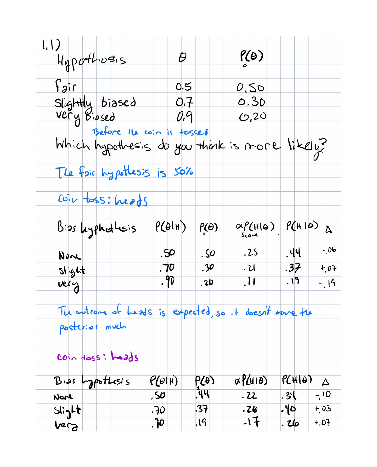
Suppose the coin’s bias could be one of three values:
| Hypothesis | Prior | |
|---|---|---|
| fair | 0.5 | 0.50 |
| slightly biased | 0.7 | 0.30 |
| very biased | 0.9 | 0.20 |
After observing heads, compute
for each hypothesis.
These are not yet posterior probabilities. They are unnormalized scores.
That distinction matters because the multiplication step compares hypotheses, while the normalization step turns the comparison into a proper distribution.
Normalization Restores Probability Mass To 1
Once the scores are computed, add them together:
Then divide each score by .
This is the discrete version of the evidence term from Lesson 19. It is the bookkeeping step that makes everything sum to 1 again.
Yesterday’s Posterior Becomes Today’s Prior
This is the deepest practical idea in the lesson:
You do not restart from scratch after each observation.
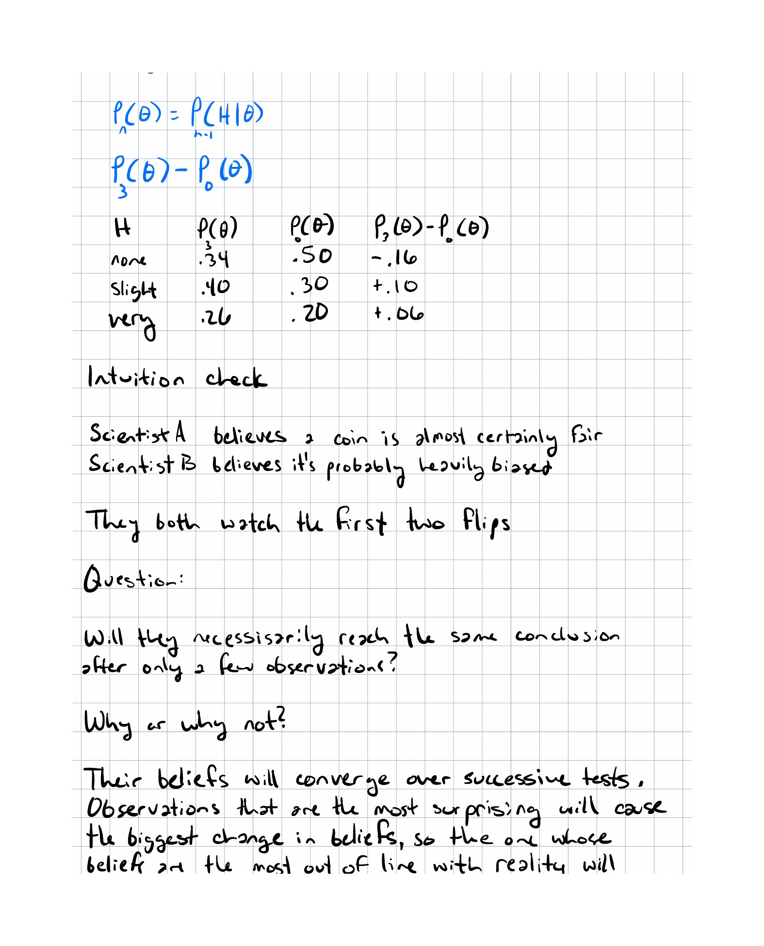
If one observation has already been processed, the posterior from that update becomes the prior for the next one:
That is why Bayesian updating naturally supports streaming data and repeated evidence accumulation.
Evidence Changes Beliefs In Proportion To Surprise
An observation is informative when it separates hypotheses.
If every hypothesis predicted heads almost equally well, then the posterior changes only a little.
If one hypothesis predicted the observation much better than the others, then the posterior shifts more dramatically.
That gives a good intuition for evidence:
Evidence matters to the extent that it changes the relative plausibility of competing explanations.
Priors Can Differ At First And Still Converge Later
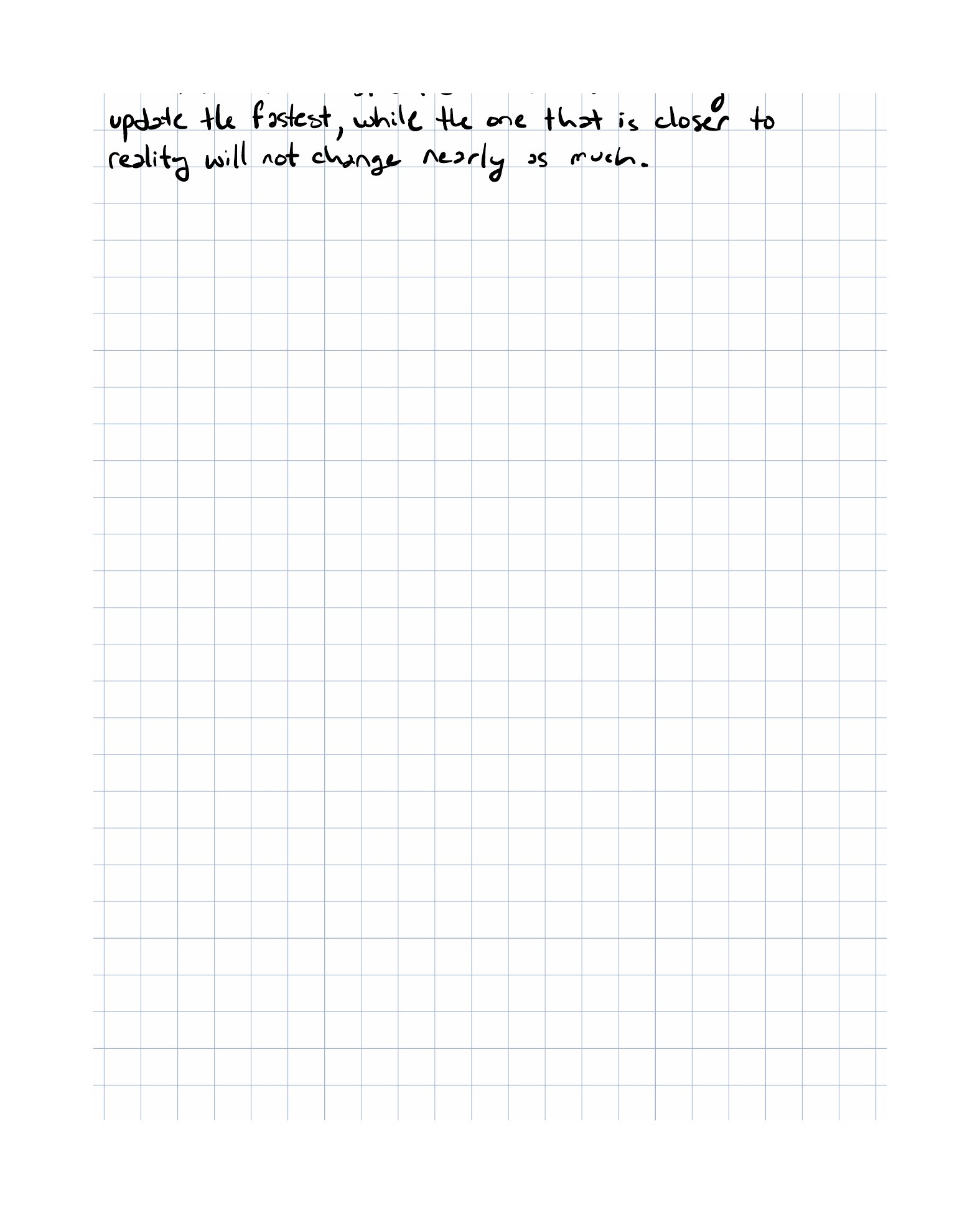
Two scientists can watch the same data and still have different posteriors after a small number of observations because they started from different priors.
As more data arrives, those prior differences often matter less, provided neither scientist assigned zero probability to the truth.
This makes room for two ideas at once:
- early beliefs matter,
- sustained evidence can overpower reasonable prior disagreement.
Worked Example
Use the three coin-bias hypotheses from above and observe one heads result.
First compute the scores:
- fair:
- slightly biased:
- very biased:
These sum to
Now normalize:
The fair hypothesis is still most probable, but less so than before. One heads result was not strong enough to erase the prior advantage, yet it did nudge mass toward more biased hypotheses.
That is the right qualitative reading:
A single unsurprising observation causes only a modest update.
Why This Shows Up In ML
Machine learning systems often process information incrementally:
- online learning updates after new samples arrive,
- filtering methods revise beliefs as new sensor data appears,
- stochastic optimization uses repeated small corrections instead of one giant calculation.
Bayesian updating offers the conceptual template for that pattern:
- keep a current belief state,
- incorporate new evidence,
- continue from the updated state.
Even when the actual training algorithm is not a fully Bayesian posterior update, this “state plus evidence plus normalization or correction” mindset shows up everywhere.
Exercises
- In the three-hypothesis coin example, why does the fair hypothesis remain largest after one heads result?
- Why are the products
prior × likelihoodnot yet a valid posterior? - If the second flip is also heads, which hypothesis should gain the most and why?
- Why can two scientists with different priors disagree after a few observations but become more similar after many observations?
- What goes wrong if a prior assigns exact probability zero to the true hypothesis?
Implementation Exercise
Implement one Bayesian update step for a finite hypothesis set in TypeScript:
type Hypothesis = {
  theta: number;
  probability: number;
};

const updateAfterHeads = (hypotheses: Hypothesis[]): Hypothesis[] => {
  const scored = hypotheses.map(({ theta, probability }) => ({
    theta,
    score: probability * theta,
  }));

  const total = scored.reduce((sum, { score }) => sum + score, 0);

  return scored.map(({ theta, score }) => ({
    theta,
    probability: score / total,
  }));
};
Run the function repeatedly for several heads observations and track how the distribution evolves over time. Then repeat with a tails observation and describe how the update direction changes.
Reflection Questions
- Which part of the update now feels most intuitive: multiplying, normalizing, or reusing the posterior?
- What kind of evidence would produce a dramatic update instead of a mild one?
- Why is sequential updating such a natural fit for computation?
- How does this lesson change your understanding of what it means for evidence to “pay rent”?
Completed Exercises
Handwritten work submitted after completing this lesson.