Lesson 21: Bayesian Predictive Distributions

Goal

Understand the Bayesian shift from estimating a single unknown parameter to predicting future observations by averaging over many plausible parameter values.

The core idea is:

A Bayesian does not usually say “this one parameter value is the truth.” A Bayesian says “these parameter values are plausible, with different weights, so predictions should average across them.”

Motivation

The previous Bayesian lessons focused on updating beliefs about an unknown parameter:

prior
likelihood
posterior

That answers a parameter question:

Given the data, what do I believe about θ now?

Machine learning usually needs the next question:

Given the data, what do I expect to observe next?

Those are not the same question. A single parameter estimate can be useful, but it throws away uncertainty. Bayesian prediction keeps that uncertainty alive long enough to influence the forecast.

Prerequisites

Lesson 18: MAP Estimation.
Lesson 19: Bayesian Estimation Introduction.
Lesson 20: Bayesian Estimation Update.
Basic comfort with probabilities, likelihoods, and the idea that a model parameter controls a distribution.

Notation / Symbol Table

Symbol	Plain-English name	Meaning
`θ`	parameter	The unknown model parameter or hypothesis.
`D`	data	The observations we have already seen.
`P(θ)`	prior	Beliefs about `θ` before seeing the data.
`P(D	θ)`	likelihood
`P(θ	D)`	posterior
`x_next`	next observation	The future value we want to predict.
`P(x_next	θ)`	one-model prediction
`P(x_next	D)`	posterior predictive

The posterior predictive distribution is

P(x_{\text{next}} \mid D) = \int P(x_{\text{next}} \mid \theta) P(\theta \mid D)\, d\theta.

Read that as:

For each possible parameter value, ask what it predicts, then average those predictions using the posterior weights.

Core Ideas

Prediction Is Not The Same As Estimation

A frequentist plug-in prediction often looks like this:

P(x_{\text{next}}) = P(x_{\text{next}} \mid \hat{\theta}),

where θ̂ is a single estimate such as the MLE or MAP estimate.

That can work well when uncertainty is tiny. But if many parameter values are still plausible, choosing one of them pretends the uncertainty disappeared.

Bayesian prediction keeps the full posterior:

P(\theta \mid D),

then uses it to build a prediction.

The Posterior Predictive Is Model Averaging

Each possible θ acts like a small model. Some models get high posterior weight. Others get low weight.

The posterior predictive combines them:

P(x_{\text{next}} \mid D) = \int P(x_{\text{next}} \mid \theta) P(\theta \mid D)\, d\theta.

This is often called model averaging. Instead of saying “Model B barely beat Model A, so ignore A,” we say “both are plausible, so both should influence the prediction.”

Why Uncertainty Matters

Suppose the posterior has two strong peaks. Then the “middle” parameter value may not actually be the most plausible one.

That means choosing one representative parameter can be misleading. Averaging predictions is usually safer than pretending a single point estimate captures the whole story.

This becomes especially important when:

the dataset is still small
several hypotheses explain the data almost equally well
future decisions depend on uncertainty, not only the most likely outcome

A Helpful Geometric Analogy

There is a useful analogy to weighted combinations from linear algebra.

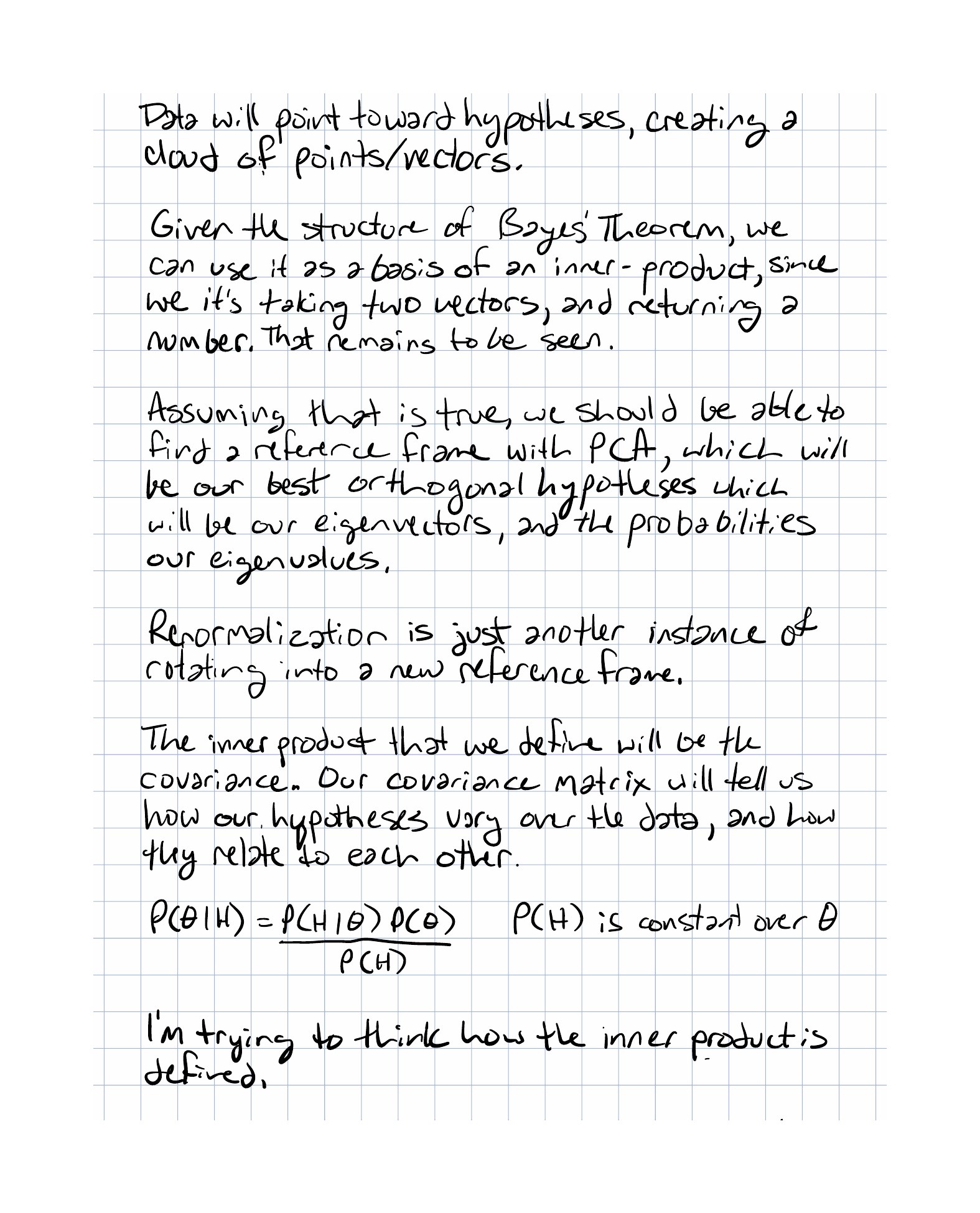
When you write a vector as a weighted combination of basis vectors, the weights tell you how much each direction contributes. A posterior does something structurally similar: it forms a weighted combination of hypotheses.

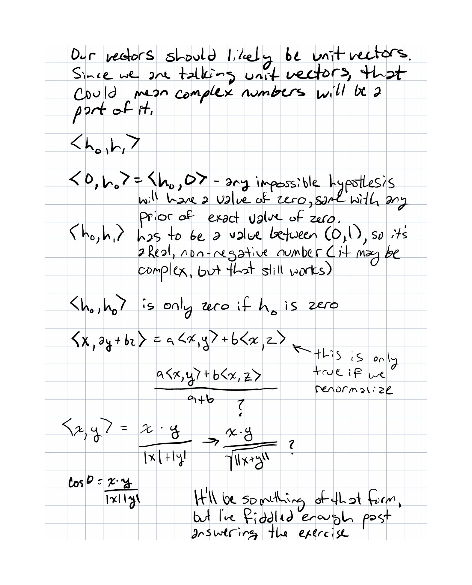
That analogy is helpful, but it has limits. Probability distributions are not ordinary vectors. The weights must stay nonnegative and sum to one. So the cleaner mental model is:

A posterior is a convex combination of hypotheses, and the posterior predictive is the corresponding weighted average of their predictions.

What Happens When The Posterior Gets Narrow

If the posterior becomes sharply concentrated around one value, then Bayesian prediction starts to look like plug-in prediction.

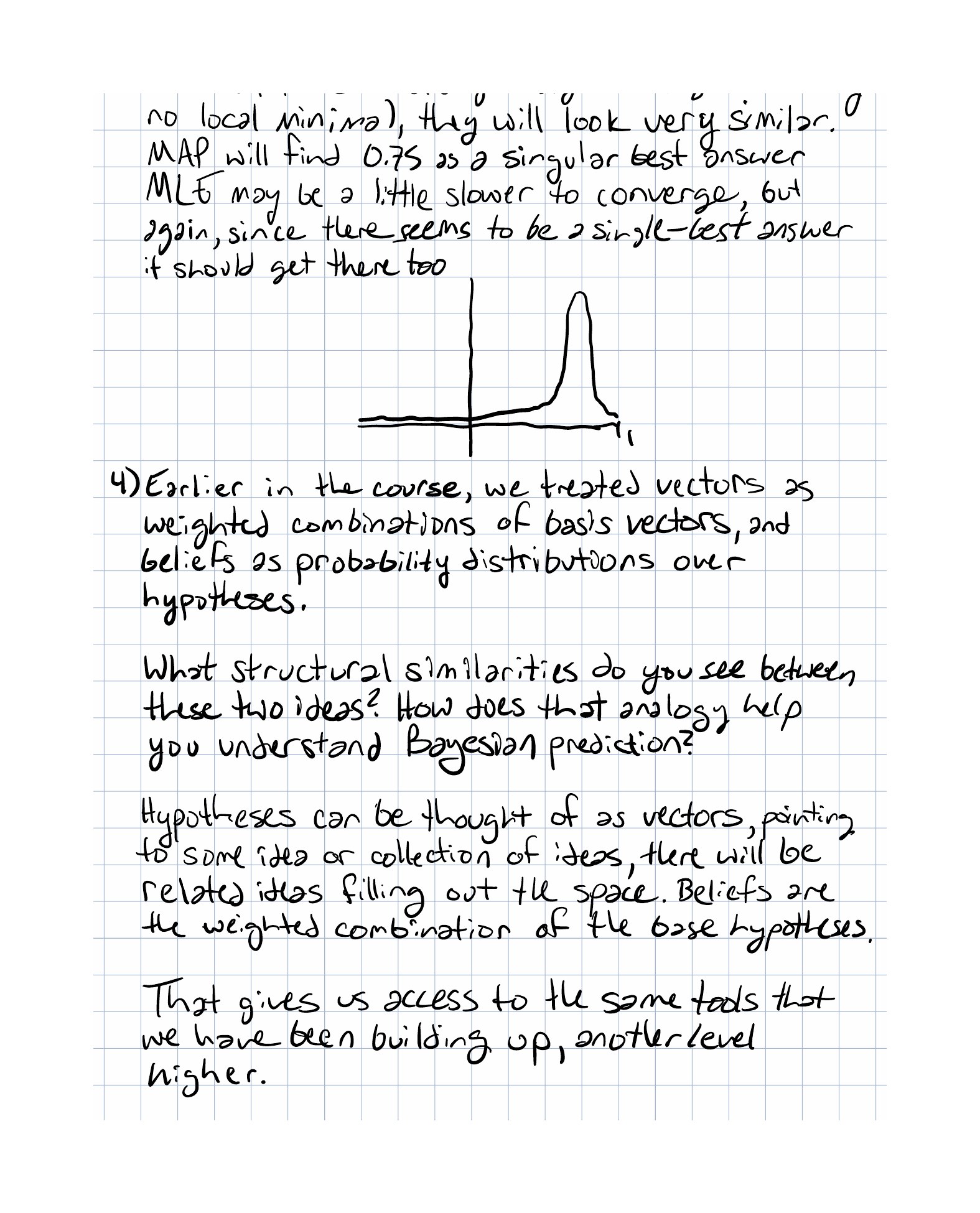
Formally, if almost all posterior mass is near θ = 0.75, then

P(x_{\text{next}} \mid D)

becomes very close to

P(x_{\text{next}} \mid \theta = 0.75).

So Bayesian and classical predictions often look similar when the data is abundant and uncertainty is small.

Worked Example

Example 1: Weather Models

Suppose three forecasting models are still plausible after seeing the available data:

Model	Posterior weight	Predicted temperature
A	0.5	70°F
B	0.3	75°F
C	0.2	80°F

A winner-take-all prediction would choose Model A and predict 70°F.

A posterior predictive average gives

0.5(70) + 0.3(75) + 0.2(80) = 73.5.

The point is not that 73.5 must be the exact truth. The point is that the prediction remembers uncertainty instead of deleting it.

Example 2: Predicting The Next Coin Flip

Suppose the posterior over the coin-bias parameter θ is:

`θ`	Posterior probability
0.3	0.2
0.5	0.5
0.7	0.3

For a Bernoulli model, each hypothesis predicts

P(H \mid \theta) = \theta.

So the posterior predictive probability of heads is

P(H_{\text{next}} \mid D) = 0.2(0.3) + 0.5(0.5) + 0.3(0.7).

Compute it:

0.06 + 0.25 + 0.21 = 0.52.

So the next-flip prediction is

P(H_{\text{next}} \mid D) = 0.52.

We never had to declare one single value of θ to be the whole story.

Why This Shows Up In ML

Machine learning systems often care about more than a best-fit parameter vector. They care about prediction under uncertainty.

Posterior predictive reasoning shows up when you:

average predictions from several plausible models
use Bayesian linear regression or Gaussian-process style reasoning
want calibrated uncertainty instead of only a point prediction
prefer robust forecasts when data is limited

Even outside fully Bayesian pipelines, the intuition survives. Ensembles, bagging, and model averaging all echo the same lesson:

Combining several plausible predictors is often better than trusting a single brittle winner.

Exercises

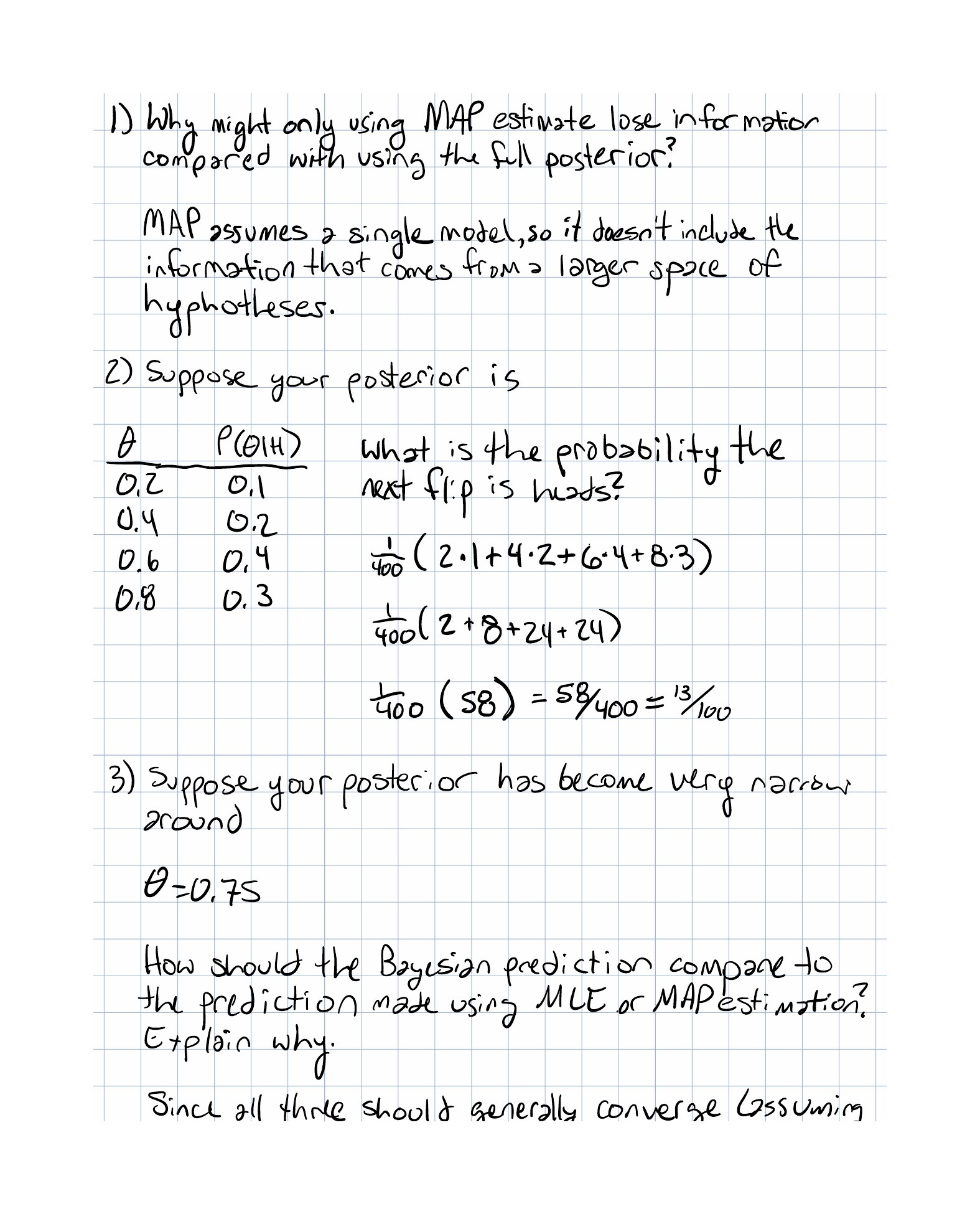
Why does using only the MAP estimate lose information compared with using the full posterior?
Suppose the posterior over a coin bias is 0.1 on θ = 0.2, 0.2 on θ = 0.4, 0.4 on θ = 0.6, and 0.3 on θ = 0.8. What is the posterior predictive probability of heads?
If the posterior becomes extremely narrow around θ = 0.75, why should Bayesian, MAP, and MLE-based predictions begin to look similar?
In what sense is a posterior like a weighted combination of hypotheses, and where does that analogy stop being exact?

Implementation Exercise

Write a TypeScript helper that computes a discrete posterior predictive distribution from a list of weighted hypotheses.

Use a shape like:

type HypothesisPrediction = {
  posteriorWeight: number;
  prediction: number;
};

Start with a Bernoulli example, where each hypothesis predicts the probability of heads. Then extend it so a hypothesis can return a small discrete probability table for outcomes like sunny, cloudy, and rainy.

The useful habit here is not just summing numbers. It is naming the pieces clearly:

one hypothesis
its posterior weight
its prediction
the final weighted average

Reflection Questions

When is a single best parameter estimate enough, and when is it too aggressive a simplification?
Why is a posterior predictive distribution more honest than a plug-in estimate when uncertainty is still large?
Which part of the formula felt most intuitive: the hypothesis-specific prediction or the averaging step?
How would you explain model averaging to someone who only knows ordinary weighted averages?

Completed Exercises

Handwritten work submitted after completing this lesson.