Goal
Understand model complexity as a tradeoff: more expressive models can fit the training data better, but that same flexibility can make them memorize noise instead of learning the underlying pattern.
Motivation
After the Bayesian lessons, it is tempting to think the hard part of machine learning is only estimating parameters well. But there is a more basic question underneath parameter estimation:
What kind of model are we even fitting?
If the model family is too simple, it misses real structure. If it is too flexible, it can chase accidental quirks of the training data. This lesson introduces the vocabulary for that tradeoff.
Prerequisites
- Lesson 17: Loss Functions.
- Lesson 21: Bayesian Predictive Distributions.
- Familiarity with straight lines, polynomials, and the idea that data may contain randomness.
Notation / Symbol Table
| Symbol | Plain-English name | Meaning |
|---|---|---|
x | input | The feature or independent variable. |
y | output | The observed target value. |
f(x) | signal | The underlying relationship we wish to learn. |
ε | noise | Random variation or measurement error. |
σ² | noise variance | How spread out the noise tends to be. |
y = f(x) + ε | signal-plus-noise model | The idea that observations contain both structure and randomness. |
Core Ideas
Data Contains Signal And Noise
A useful mental model is
where:
f(x)is the underlying patternεis random noise
Machine learning should learn f(x), not memorize ε.
That is the whole overfitting story in one line.
Complexity Means Representational Power
Different model families can represent different kinds of functions:
- a constant
- a straight line
- a quadratic
- a high-degree polynomial
- a large neural network
This is what people mean by capacity or model complexity. Higher capacity means:
I can represent more complicated relationships.
It does not mean:
I will automatically make better predictions.
Why Training Error Usually Goes Down
As complexity increases, the model gets more degrees of freedom. That usually makes it easier to reduce training error.
This is why a high-capacity model often looks impressive on the dataset it already saw. It has enough flexibility to explain many small details, including details that do not matter outside that dataset.
The Three Regimes
There are three standard regions to keep straight.
Underfitting:
- the model is too simple
- training error is high
- test error is also high
Good fit:
- the model captures the main structure
- training error is low
- test error is also low
Overfitting:
- the model memorizes training quirks
- training error becomes extremely small
- test error gets worse
The key point is that the best generalizing model is not necessarily the one with the smallest training error.
Generalization Is The Real Objective
Machine learning is not a contest to explain the past perfectly. It is a contest to perform well on unseen data.
That is what generalization means:
How well does the model behave on examples it did not memorize during training?
This is why we eventually need validation and test sets. We need some way to check whether the learned rule transfers beyond the training sample.
A Small Mathematical Correction Worth Keeping
In the original transcript, one thought experiment used five points and a fifth-degree polynomial. The sharper mathematical statement is:
For five distinct points, the unique interpolating polynomial has degree at most four.
A fifth-degree polynomial can still pass through the points, but then it is no longer unique. That detail does not change the lesson’s intuition. It just keeps the algebra honest.
Worked Example
Example 1: A Line Versus A Highly Flexible Polynomial
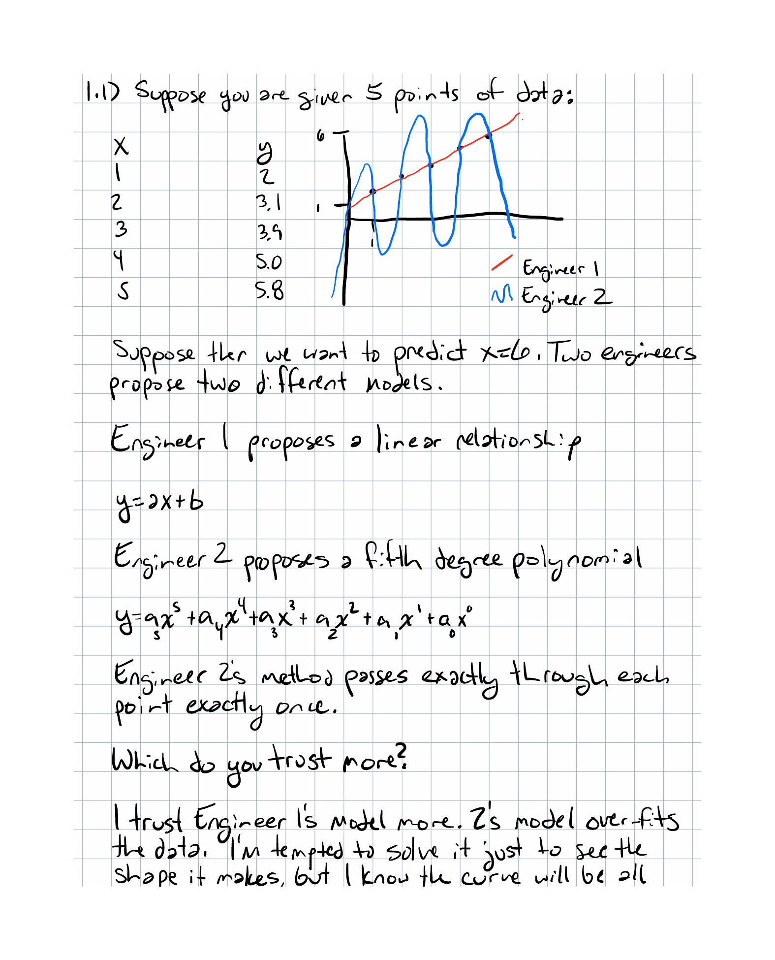
Suppose we observe:
x | y |
|---|---|
| 1 | 2.0 |
| 2 | 3.1 |
| 3 | 3.9 |
| 4 | 5.0 |
| 5 | 5.8 |
Now compare two model families:
- Model A: a straight line,
y = ax + b - Model B: a high-degree polynomial that hits every point exactly
Model B can drive training error to zero. That sounds impressive, but zero training error is not proof of good prediction. If the underlying process is roughly linear with noise, the extra wiggle is probably noise-fitting.
The sensible question is:
Which model would you trust more at
x = 6?
That is a generalization question, not a training-error question.
Example 2: Two Accuracy Reports
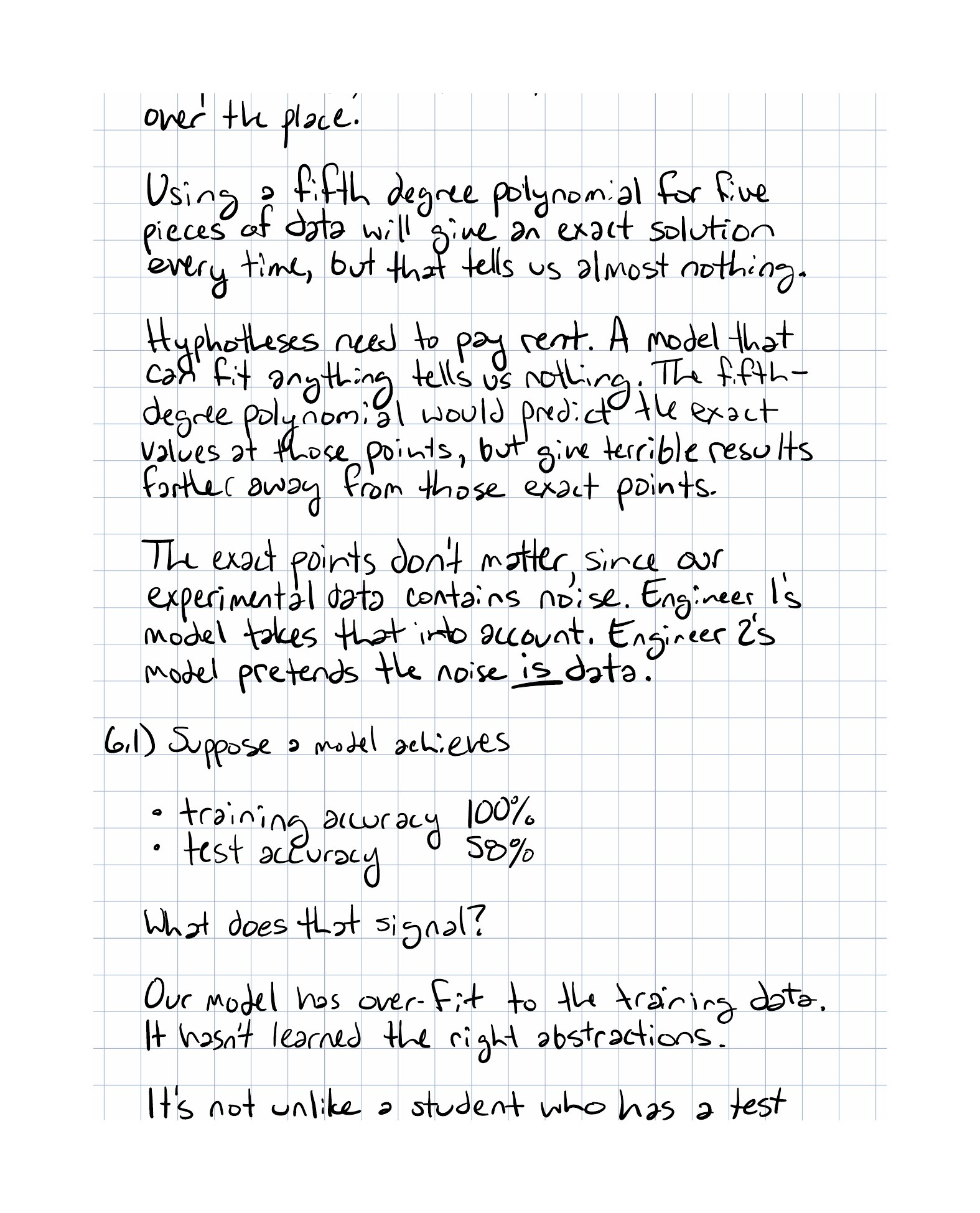
Suppose one model achieves:
- training accuracy:
100% - test accuracy:
58%
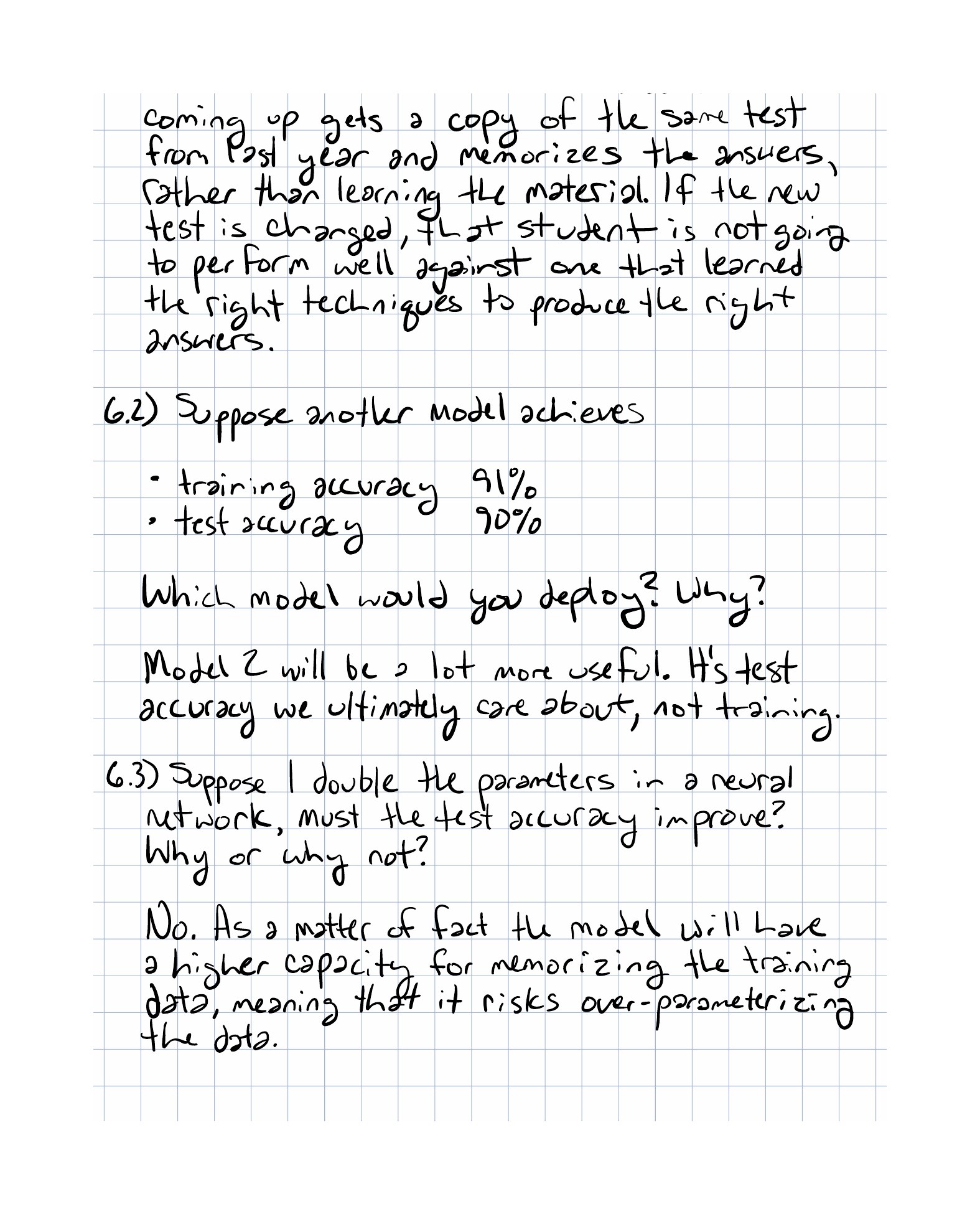
and another achieves:
- training accuracy:
91% - test accuracy:
90%
The second model is usually the one you would deploy. It has learned a rule that transfers.
This is the habit to build early:
Treat perfect training performance with suspicion unless unseen-data performance confirms it.
Why This Shows Up In ML
Every serious ML workflow faces complexity choices:
- how many features to include
- how deep or wide the network should be
- what basis functions to allow
- whether to use a simpler or richer model family
The lesson also sets up several later tools:
- regularization, which discourages overly flexible solutions
- early stopping, which avoids memorization during optimization
- validation sets, which help choose complexity without touching the final test set
If you remember one sentence, make it this one:
Low training error tells you the model can explain the data it saw. Generalization tells you whether that explanation survives contact with new data.
Exercises
- Why can a model with more parameters fit the training data better without necessarily improving test performance?
- Explain the difference between signal and noise in the expression
y = f(x) + ε. - Describe the behavioral difference between underfitting and overfitting without using formulas.
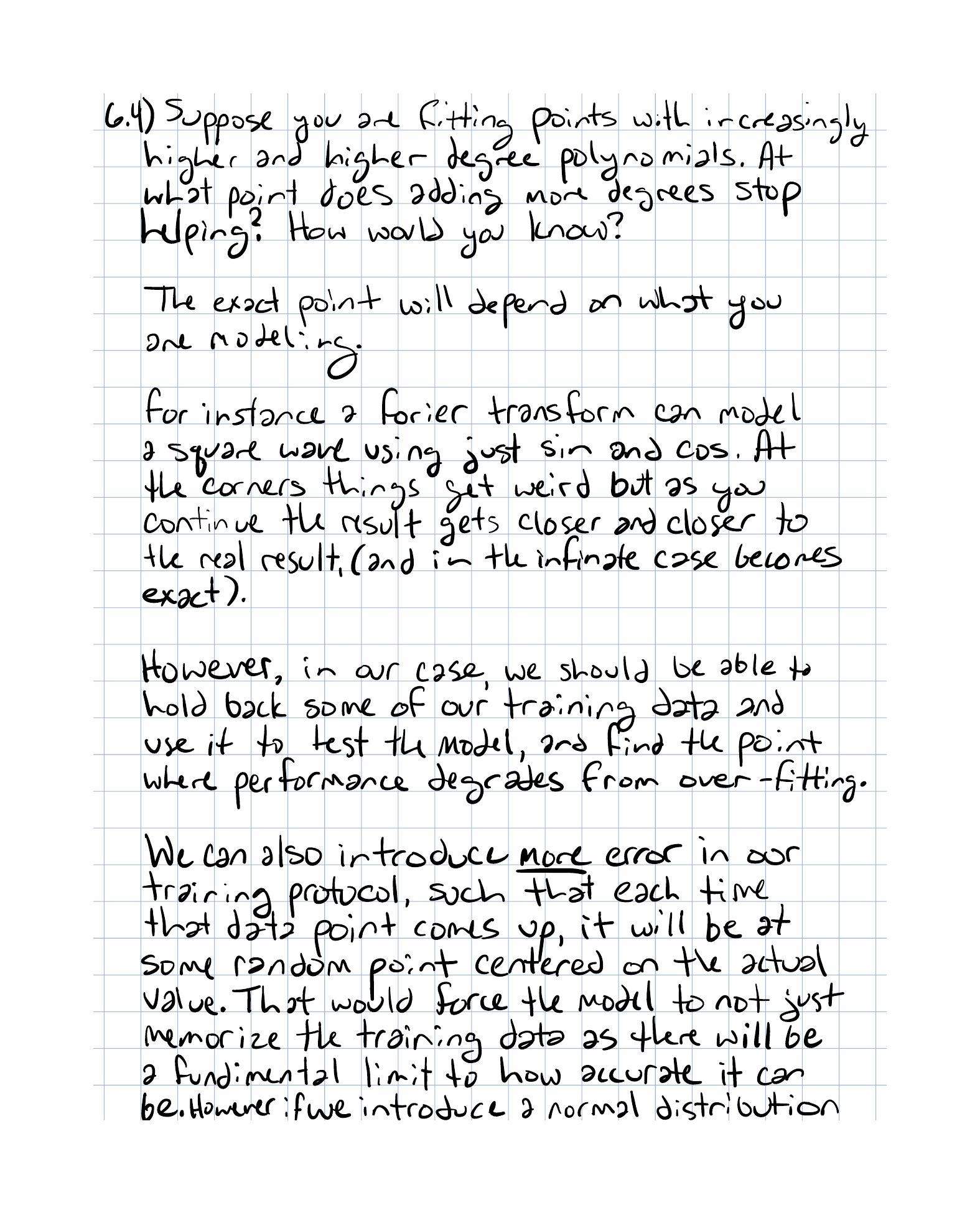
- Suppose adding more polynomial degrees keeps reducing training error. How would you decide when those extra degrees stop helping?
Implementation Exercise
Build a small TypeScript experiment that generates noisy points from a simple rule such as
then compares several model families on separate training and validation splits.
A good version of the exercise should record:
- the model family or degree
- training error
- validation error
- which degree gives the best validation performance
You do not need a fancy plotting library to learn something here. Even a printed table is enough to make the pattern visible.
Reflection Questions
- Why is “fits the data perfectly” not the same as “understands the process”?
- Which feels more natural to you right now: thinking in terms of capacity, or thinking in terms of signal versus noise?
- When have you seen a software system become too complex for the problem it was solving?
- What would convince you that a simpler model is actually better than a more impressive-looking one?
Completed Exercises
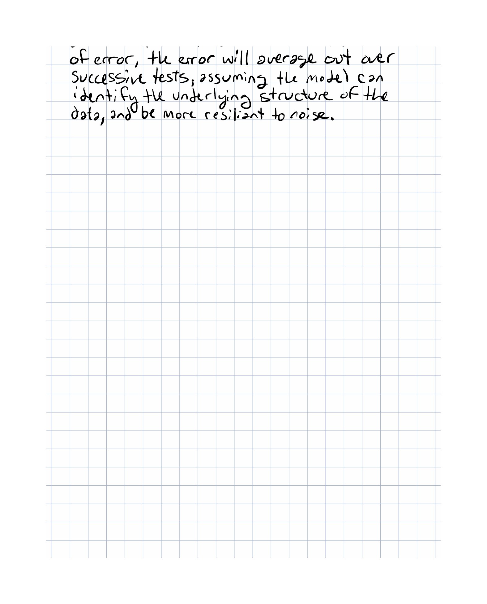
Handwritten work submitted after completing this lesson.