Goal
Understand regularization as adding a second goal to learning: fit the data, but prefer parameter values that stay simple enough to generalize.
Motivation
Lesson 22 introduced the problem: high-capacity models can memorize noise. Regularization is one of the cleanest responses to that problem.
Instead of asking only
How well does the model fit the observed data?
we also ask
Among models with similar fit, which ones are less brittle?
That extra preference changes the optimization problem in a useful way.
Prerequisites
- Lesson 17: Loss Functions.
- Lesson 18: MAP Estimation.
- Lesson 22: Model Complexity.
- Comfort with the idea that weights or coefficients control a model’s behavior.
Notation / Symbol Table
| Symbol | Plain-English name | Meaning |
|---|---|---|
w | weight vector | The model parameters we are learning. |
λ | lambda | How strongly we penalize complex parameter choices. |
| ` | w | |
| ` | w | |
Loss_data(w) | data-fit term | The part of the loss that measures prediction error on the training data. |
Loss_data(w) + λR(w) | regularized objective | The total objective, where R(w) is a penalty term. |
Core Ideas
Fitting Error Alone Is Too Permissive
If the loss function only measures training error, it has no opinion about the size of the parameters.
That means it may choose:
- small, stable coefficients
- huge, twitchy coefficients
as long as the training fit looks good.
This is one reason overfit polynomial models often come with large coefficients. The objective function never told them not to.
Regularization Adds Another Preference
The regularized pattern is:
where:
Loss_data(w)measures fit to the observed dataR(w)measures some notion of parameter size or complexityλsets the tradeoff
When λ = 0, we recover the unregularized objective.
As λ increases, the optimizer cares more about keeping the parameters small or sparse.
Why Large Weights Often Signal Brittleness
Large coefficients can make a model extremely sensitive to tiny changes in the input.
That is the geometric picture to keep:
Big weights can make nearby inputs produce very different outputs.
If the input contains noise, that sensitivity can amplify the noise into unstable predictions.
L2 Regularization Shrinks
L2 regularization uses
Because the weights are squared, very large weights are punished especially strongly.
The effect is usually:
- many weights stay nonzero
- their magnitudes get pulled downward
This is why L2 often feels like:
Spread the work across many smaller coefficients.
L1 Regularization Encourages Sparsity
L1 regularization uses
This creates a different preference. L1 is more willing to drive some weights exactly to zero.
That is why L1 often feels like:
Use as few coefficients as possible.
This becomes valuable when feature selection matters.
Lambda Controls The Tradeoff
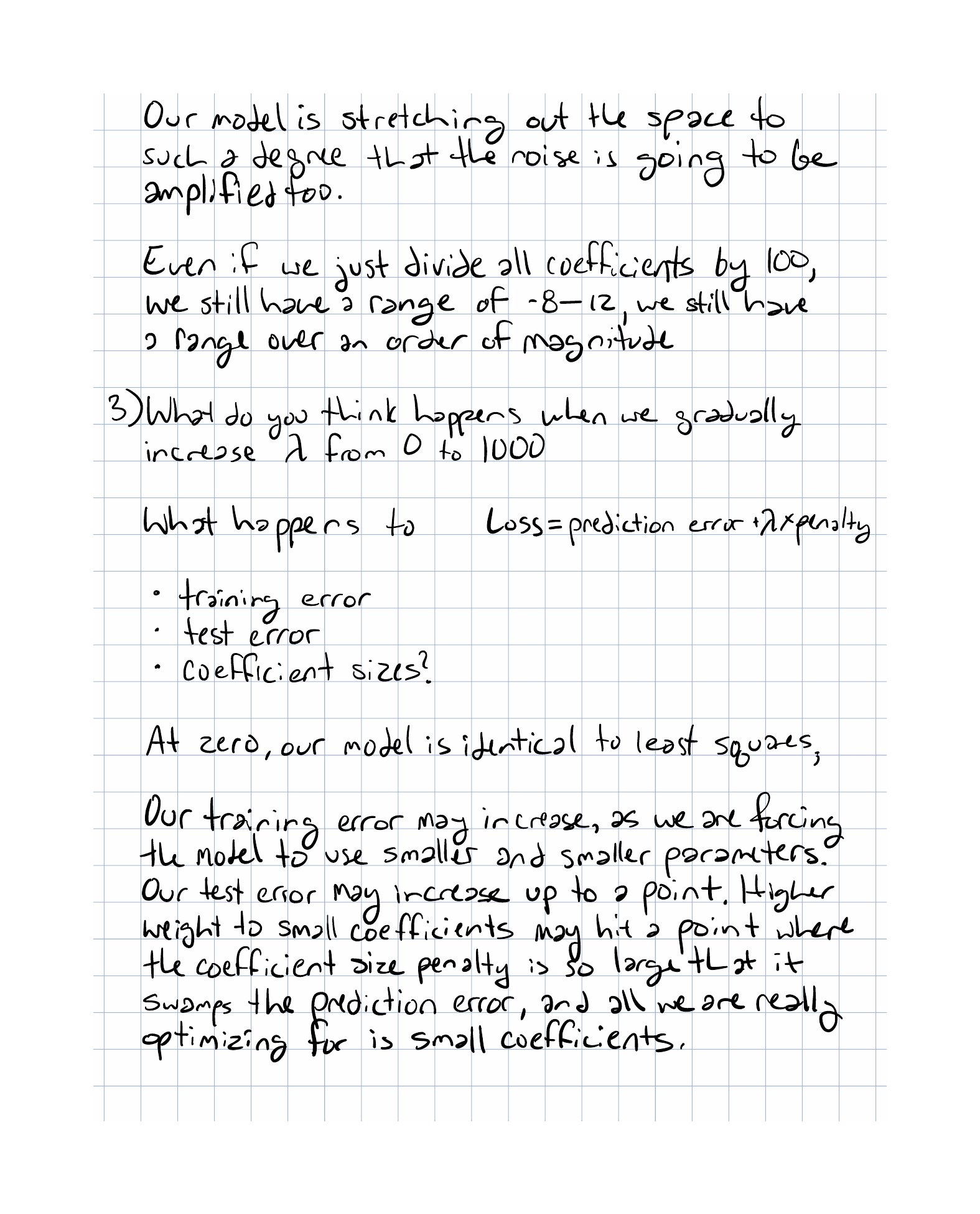
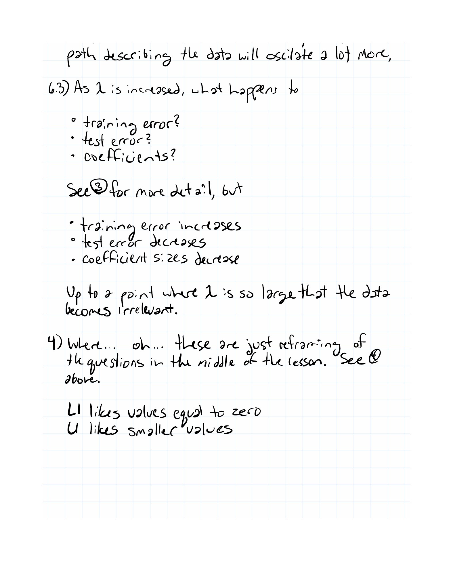
As λ increases:
- training error usually goes up
- coefficient magnitudes go down
- test error often decreases at first, then increases later
That last point matters. The common pattern is not “more regularization always helps.” It is:
Too little regularization can overfit, and too much regularization can underfit.
So the validation curve for test-like performance is often U-shaped with respect to λ.
Regularization Has A Bayesian Interpretation
Regularization is not only a numerical trick. It is also a way of encoding prior beliefs.
MAP estimation maximizes
If the prior says “weights are probably near zero,” the corresponding optimization problem looks like L2 regularization.
If the prior says “many weights should actually be zero,” the corresponding preference lines up with L1 regularization.
This is the key bridge:
Optimization language says “add a penalty.” Bayesian language says “add a prior.” In this lesson, those are often two views of the same structure.
Worked Example
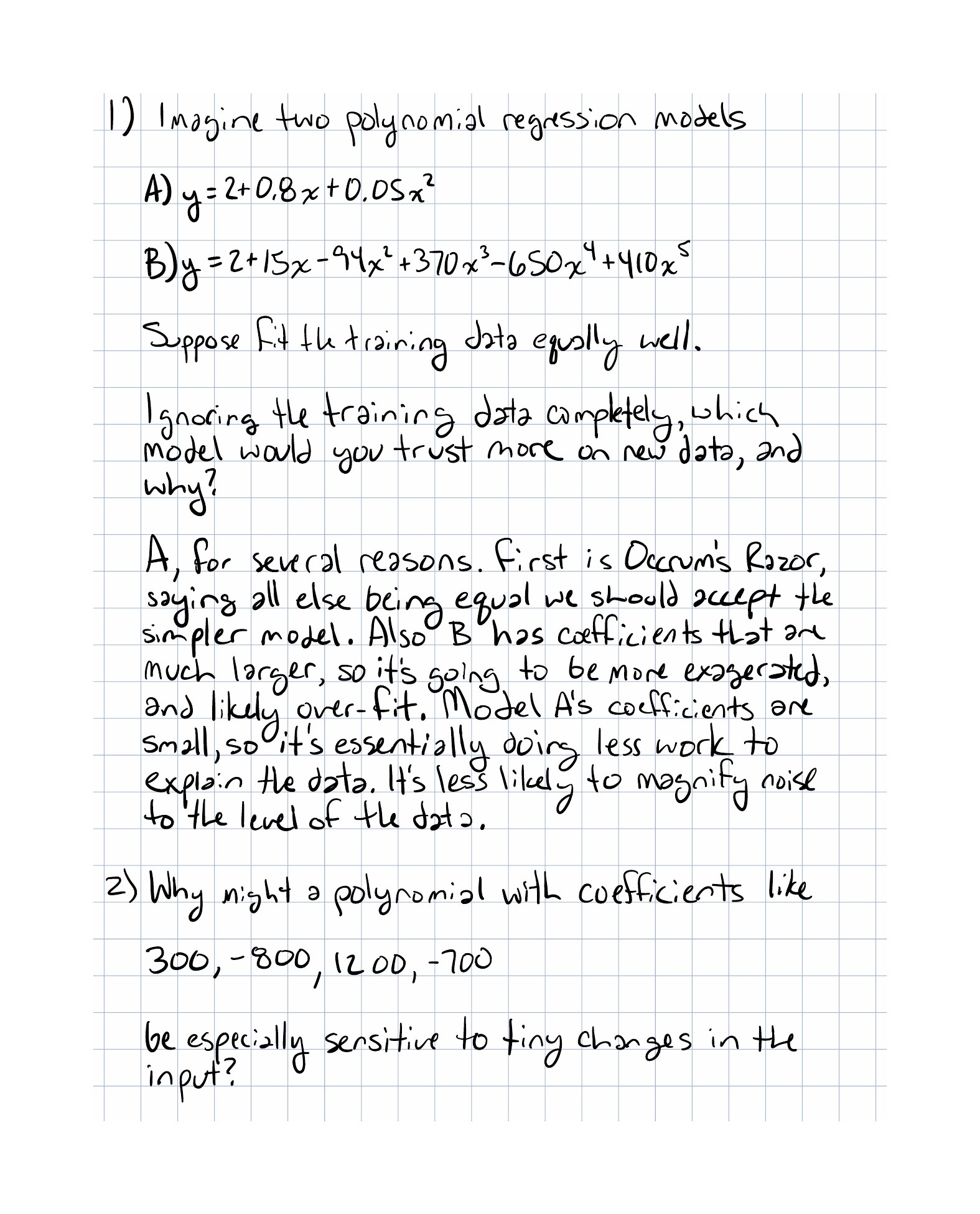
Example 1: Two Polynomial Models
Suppose we compare:
- Model A:
y = 2 + 0.8x - 0.05x² - Model B:
y = 2 + 15x - 94x² + 370x³ - 650x⁴ + 410x⁵
Even if both models fit the training data similarly, Model B is usually more fragile. Its huge coefficients suggest a function that bends sharply and reacts strongly to small input changes.
Regularization encodes a preference for Model A-like behavior unless the data gives a compelling reason to do something more extreme.
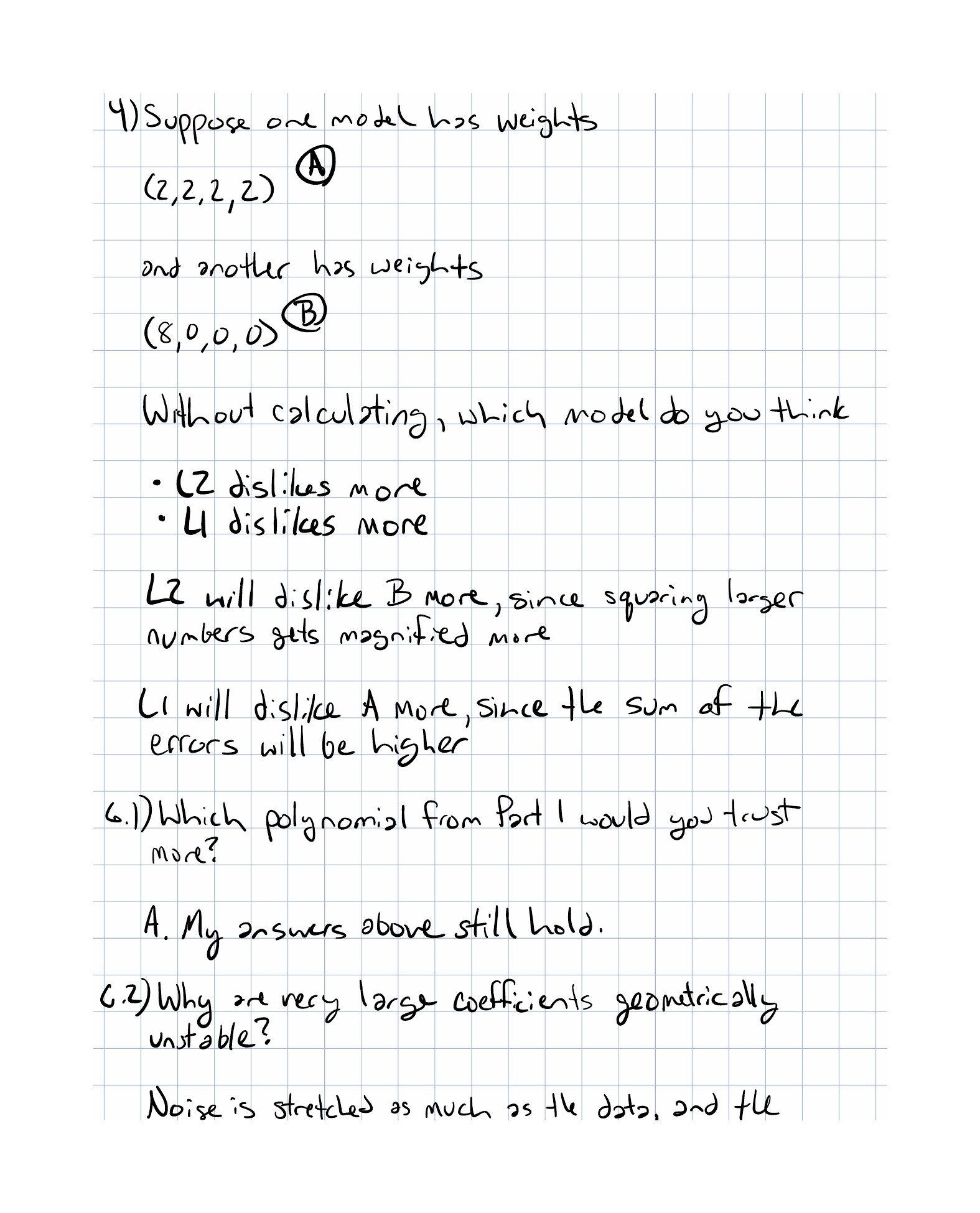
Example 2: L1 Versus L2 On Two Weight Vectors
Compare the vectors:
and
For L1:
and
So L1 treats them equally.
For L2:
while
So L2 punishes the single huge weight much more heavily.
That is a compact way to remember the difference:
- L1 is comfortable with a few exact zeros and a few active coordinates.
- L2 dislikes concentrated large weights.
Why This Shows Up In ML
Regularization appears everywhere in modern ML:
- ridge regression and weight decay
- lasso and sparse feature selection
- Bayesian priors over parameters
- neural-network training where large weights can destabilize optimization and generalization
It also provides a durable mental separation:
- the data-fit term says what counts as success on observed examples
- the penalty says what kinds of solutions we prefer among all good fits
That distinction becomes increasingly important as models get more expressive.
Exercises
- Why can a model with very large coefficients be more sensitive to noise than a model with smaller coefficients?
- What happens qualitatively to training error, test error, and weight magnitudes as
λincreases from zero to a very large value? - Why does L1 tend to produce sparse solutions more naturally than L2?
- In what sense is regularization similar to choosing a prior before seeing the data?
Implementation Exercise
Take a simple TypeScript regression experiment and extend its objective from
to
Then run the same experiment for several values of λ and record:
- training loss
- validation loss
- weight magnitudes
If you want a second pass, swap in an L1 penalty and compare how the learned weight vectors differ.
Reflection Questions
- Which interpretation lands more naturally for you right now: “penalty term” or “prior belief”?
- Why is “smaller weights” a geometric claim about stability, not just an aesthetic preference?
- When would you want weights spread across many features, and when would you want only a few active features?
- How would you explain the difference between underfitting from too much regularization and overfitting from too little?
Completed Exercises
Handwritten work submitted after completing this lesson.