Lesson 26: Gradient Descent | Mathematics of AI

Goal

Understand gradient descent as a local movement rule for minimizing a loss function: look at the current slope of the loss landscape, then move parameters in the opposite direction.

By the end of this lesson, you should be able to explain the update rule

theta_next = theta_current - learning_rate * gradient

and connect each part of that rule to geometry, loss functions, and machine learning training loops.

Gradient descent uses only local slope information. The loss defines the surface; the optimizer defines the path.

Motivation

The previous lessons built a sequence of questions:

What kind of model are we using?
What probability assumptions does the model make?
What loss function measures badness?
What regularization or stopping rule helps generalization?

Gradient descent answers the next question:

How do the parameters actually move?

Once we have a loss function, the problem becomes an optimization problem. We have a parameter vector $\theta$ , a scalar loss $L(\theta)$ , and a desire to find parameter values that make the loss small. Gradient descent is the simplest reusable movement rule:

Stand at the current parameter value.
Measure the local uphill direction.
Step downhill.
Repeat.

That is the whole idea. The power comes from the fact that the same rule works for a one-dimensional quadratic, linear regression, logistic regression, and large neural networks. The details become harder, but the invariant remains stable:

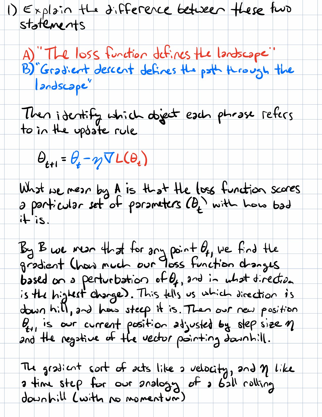
A loss function defines the landscape. An optimizer defines the path through it.

Prerequisites

Lesson 17: Loss Functions.
Lesson 23: Regularization.
Lesson 24: Early Stopping.
Lesson 25: Dropout.
Vectors, dot products, and the idea that a vector can represent model parameters.

Notation / Symbol Table

Symbol	Plain-English name	Meaning
$\theta$	parameters	The values the model can adjust during training.
$\theta_t$	current parameters	The parameter vector at optimization step $t$ .
$\theta_{t+1}$	next parameters	The parameter vector after one update.
$L(\theta)$	loss function	A scalar function measuring how bad the current parameters are.
$\nabla L(\theta_t)$	gradient at the current point	The direction of steepest local increase of the loss.
$-\nabla L(\theta_t)$	descent direction	The direction of steepest local decrease of the loss.
$\eta$	learning rate	A positive scalar controlling step size.
$\Delta \theta$	parameter update	The change added to the current parameters.
$\lVert \nabla L(\theta_t) \rVert$	gradient magnitude	How steep the loss is near the current parameters.

The basic gradient descent update is:

\theta_{t+1} = \theta_t - \eta \nabla L(\theta_t).

Read this as:

The next parameters equal the current parameters minus a scaled version of the current uphill direction.

Core Ideas

The Loss Landscape

A loss function turns parameter choices into a number:

L : \Theta \to \mathbb{R}.

For each possible parameter vector $\theta$ , the loss $L(\theta)$ tells us how bad that choice is. Low loss is good. High loss is bad.

Geometrically, you can imagine the loss as a landscape over parameter space:

In one dimension, the landscape is a curve.
In two dimensions, it is a surface.
In many dimensions, it is still a surface conceptually, even if we cannot draw it.

The optimizer does not need to see the whole landscape at once. Gradient descent is local. It asks:

At my current location, which direction increases loss fastest?

Then it moves the other way.

The Gradient Points Uphill

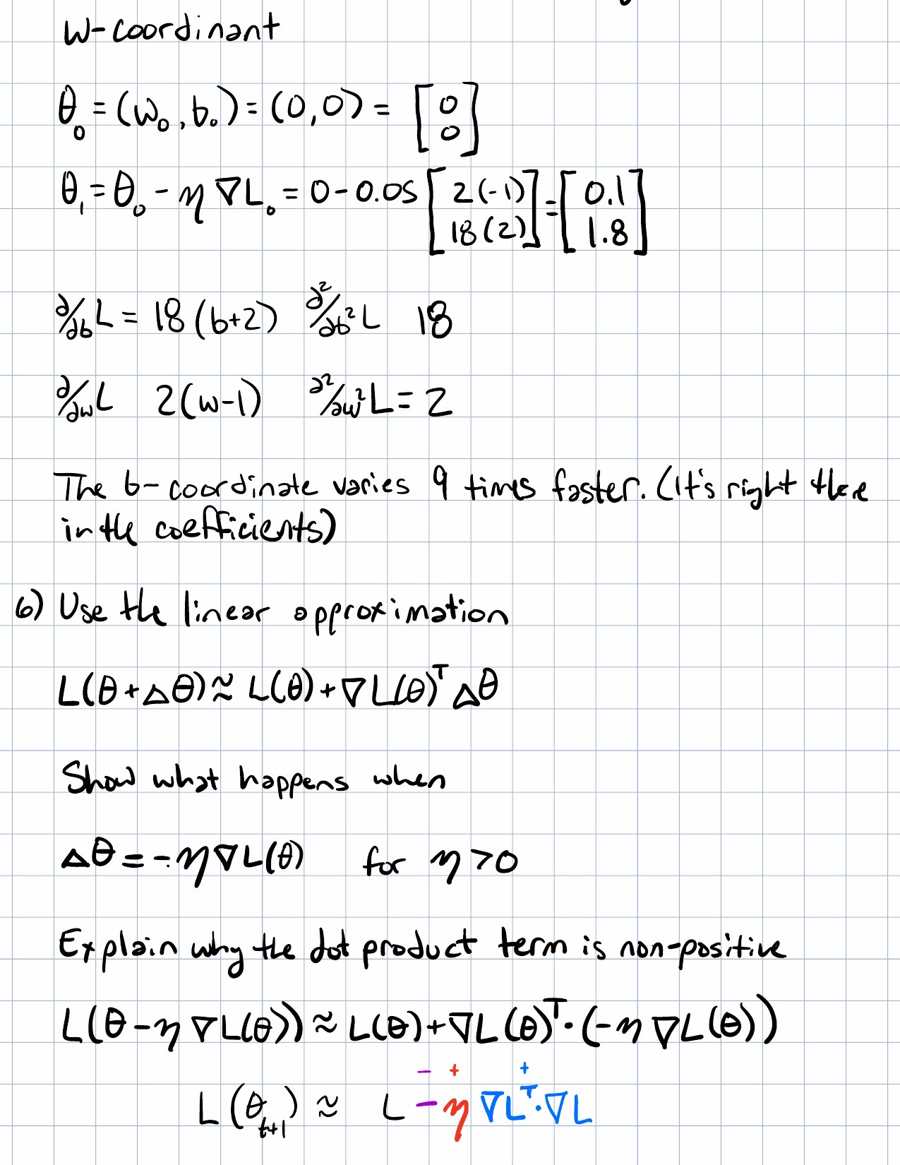
The gradient $\nabla L(\theta)$ points in the direction of steepest local increase of $L$ .

For a small movement $\Delta \theta$ , the local linear approximation is:

L(\theta + \Delta \theta) \approx L(\theta) + \nabla L(\theta)^T \Delta \theta.

The term

\nabla L(\theta)^T \Delta \theta

is a dot product. It measures how aligned your movement is with the gradient.

If $\Delta \theta$ points with the gradient, the dot product is positive and the loss increases.
If $\Delta \theta$ points against the gradient, the dot product is negative and the loss decreases.
If $\Delta \theta$ is orthogonal to the gradient, the first-order change is near zero.

This is the first important geometric compression:

Gradient descent is dot-product geometry applied to a loss landscape.

The Update Rule

Since the gradient points uphill, gradient descent moves downhill:

\Delta \theta = -\eta \nabla L(\theta_t).

Then:

\theta_{t+1} = \theta_t + \Delta \theta.

Substituting the update gives:

\theta_{t+1} = \theta_t - \eta \nabla L(\theta_t).

The minus sign is not decorative. It is the whole descent part of gradient descent.

The Learning Rate Is A Trust Scale

The learning rate $\eta$ controls how much we trust the local gradient.

A gradient is local information. It says what the loss does near the current point. It does not promise that the same direction remains good forever.

So the learning rate asks:

How far should I move before checking the slope again?

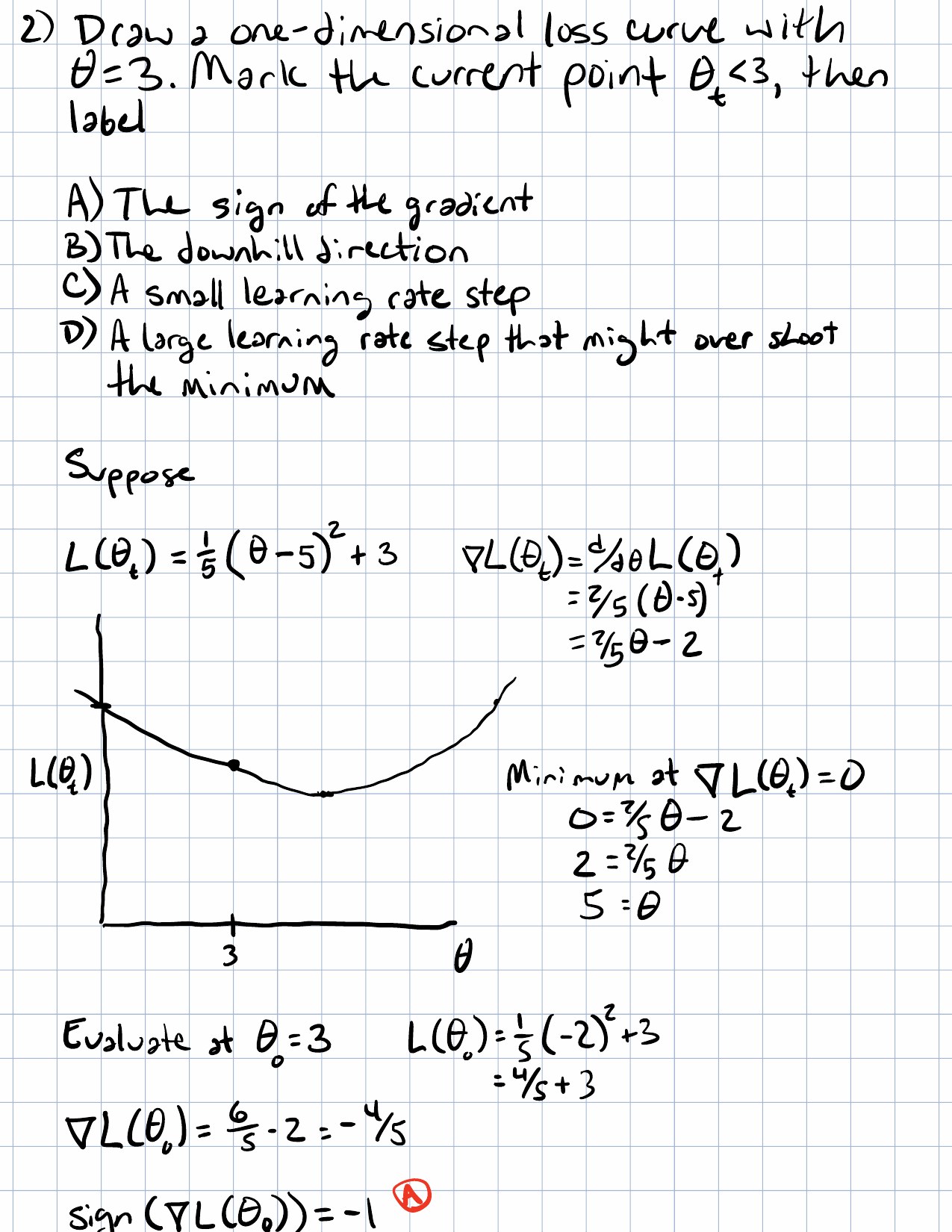
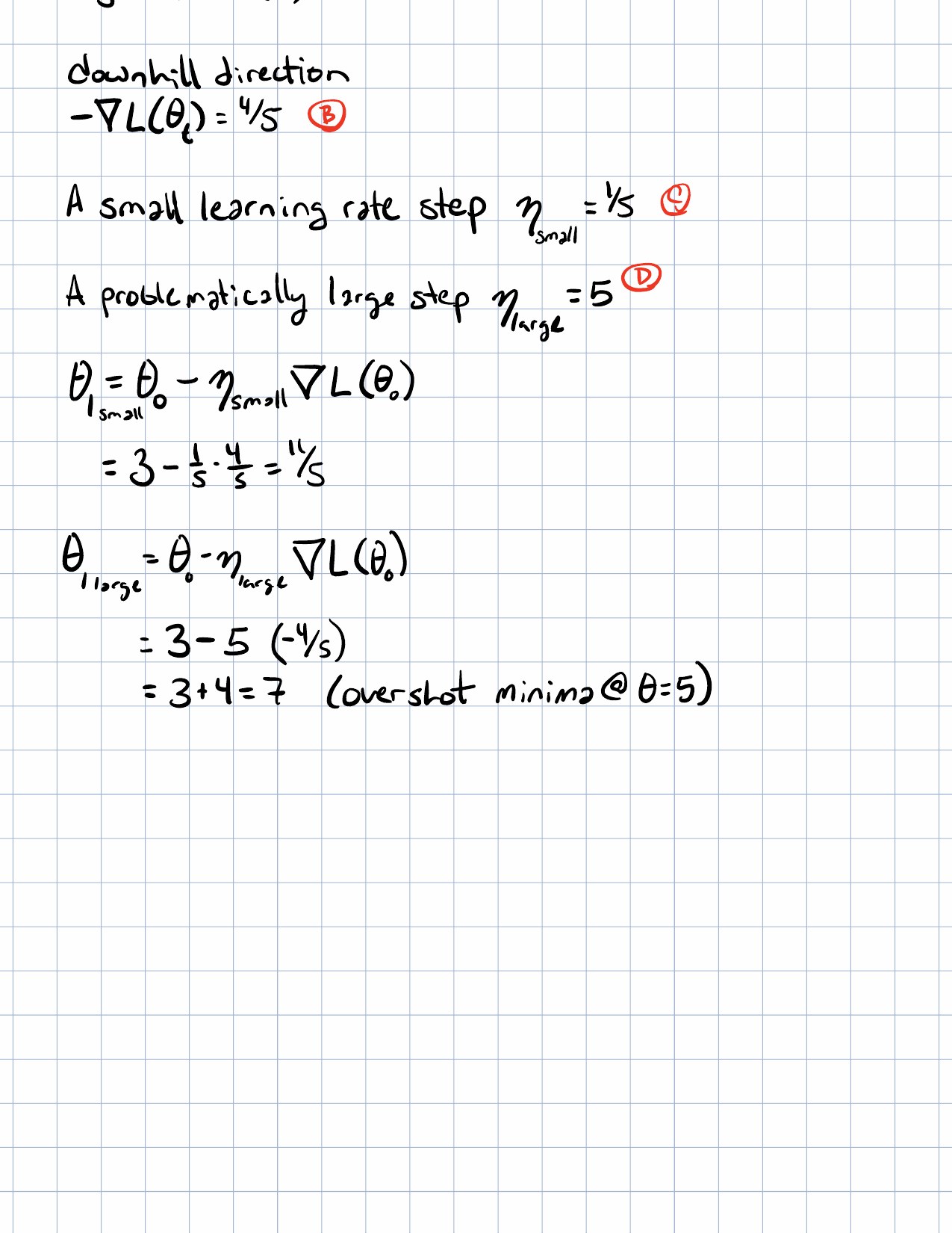
If $\eta$ is too small, training is stable but slow. If $\eta$ is too large, training can overshoot, oscillate, or diverge.

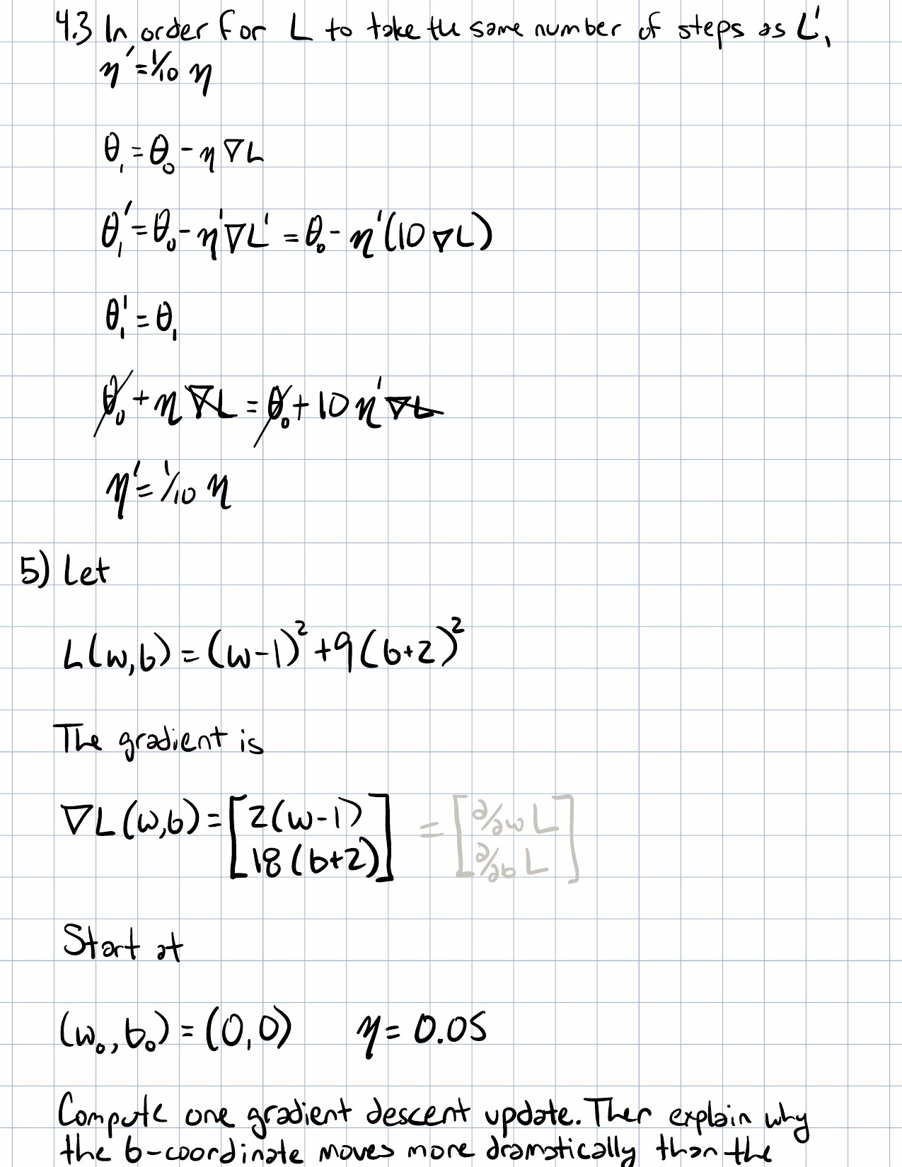
This connects directly to a point from Lesson 17. If we multiply the loss by 100:

L'(\theta) = 100L(\theta),

then:

\nabla L'(\theta) = 100\nabla L(\theta).

The minimizer has not moved, but gradient descent steps become 100 times larger unless the learning rate is adjusted.

That distinction matters:

The optimum depends on the loss landscape. The path depends on both the landscape and the optimizer settings.

Convergence Intuition

Gradient descent is usually trying to reach a point where the gradient is zero or close to zero:

\nabla L(\theta) \approx 0.

For a simple convex bowl, this means we are near the global minimum. For a nonconvex neural network landscape, it can mean a local minimum, a saddle point, or a flat region.

This is why optimization vocabulary is careful:

A minimum is a point with low loss relative to nearby points.
A global minimum is the best possible point over the whole landscape.
A local minimum is only best in its neighborhood.
A saddle point has zero gradient but is not a minimum.
Convergence means the update process has settled by some criterion.

Gradient descent does not magically know the global answer. It follows local information repeatedly.

Geometry And Conditioning

Some loss landscapes are shaped like round bowls. Others are long, narrow valleys.

In a round bowl, the same learning rate works similarly in every direction. In a narrow valley, one direction may be steep while another is shallow. A learning rate that is safe for the steep direction may be painfully slow for the shallow direction.

This should feel connected to covariance geometry:

A covariance ellipse describes different scales in different data directions.
A loss landscape can also have different scales in different parameter directions.
Optimization becomes harder when those scales are badly mismatched.

This is one reason whitening, normalization, and adaptive optimizers appear so often in machine learning. They try, in different ways, to make the geometry easier to move through.

Objective Versus Optimizer

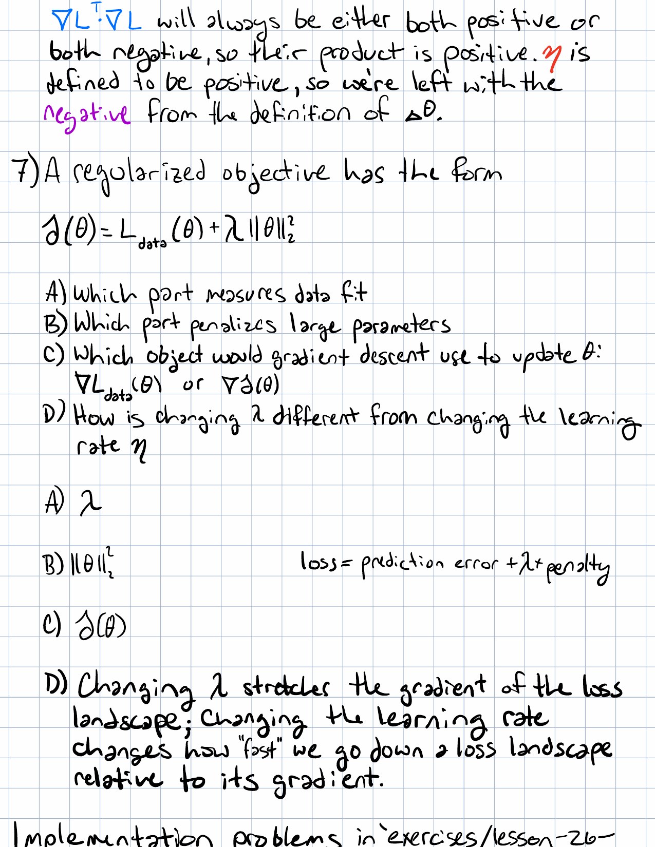
Keep these separate:

Concept	Question answered
Loss function	What are we trying to minimize?
Regularization	What parameter choices should be discouraged?
Gradient descent	How do we move through parameter space?
Learning rate	How large is each movement?
Early stopping	Which point along the path should we keep?
Dropout	How do we perturb training so representations become less brittle?

This separation prevents a common confusion. Regularization, dropout, early stopping, and gradient descent can all affect training, but they are not the same kind of object.

Worked Examples

Example 1: A One-Dimensional Quadratic

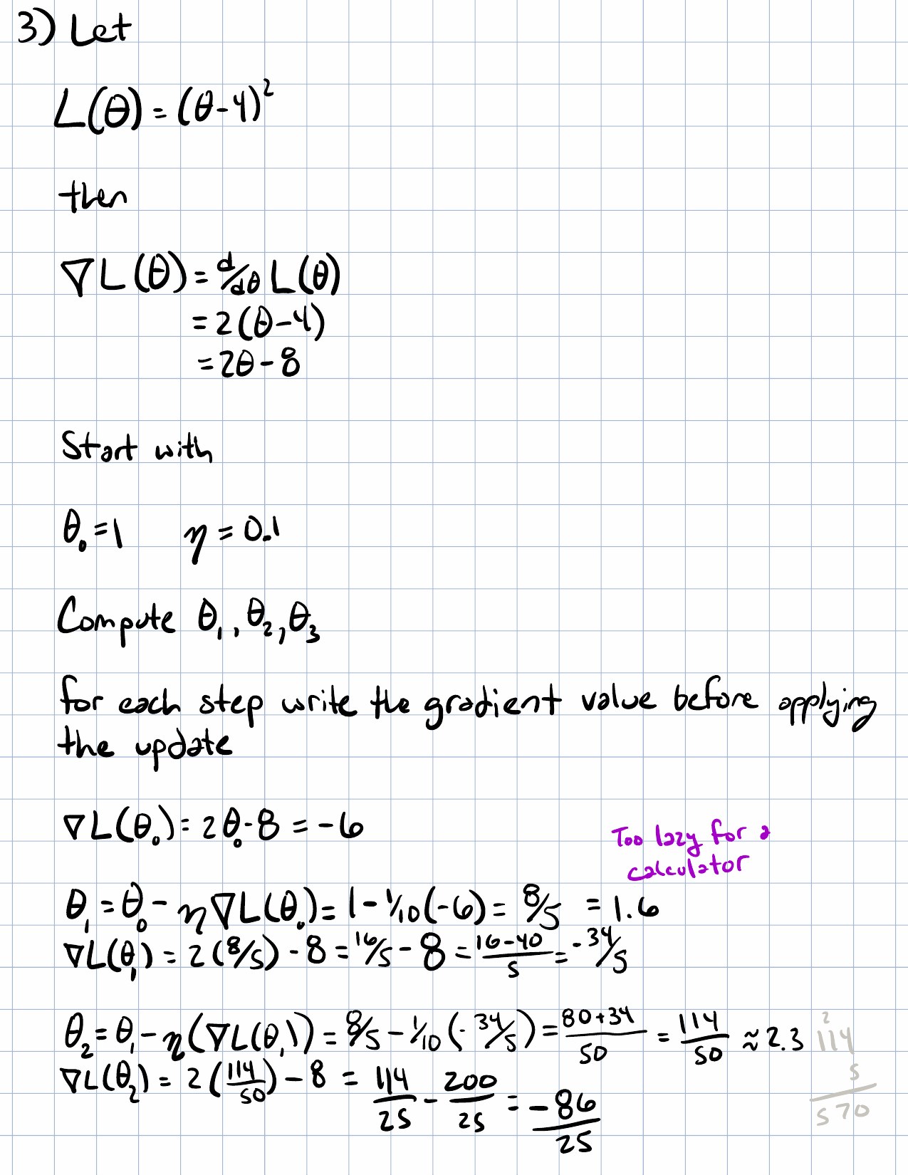
Let:

L(\theta) = (\theta - 3)^2.

This loss is minimized at $\theta = 3$ .

The gradient in one dimension is just the derivative:

\frac{dL}{d\theta} = 2(\theta - 3).

Start at:

\theta_0 = 0

and choose:

\eta = 0.1.

Step 1:

\nabla L(\theta_0) = 2(0 - 3) = -6.

\theta_1 = 0 - 0.1(-6) = 0.6.

The gradient is negative, so the downhill step moves to the right.

Step 2:

\nabla L(\theta_1) = 2(0.6 - 3) = -4.8.

\theta_2 = 0.6 - 0.1(-4.8) = 1.08.

Step 3:

\nabla L(\theta_2) = 2(1.08 - 3) = -3.84.

\theta_3 = 1.08 - 0.1(-3.84) = 1.464.

The steps get smaller as $\theta$ approaches 3 because the slope gets smaller.

Example 2: A Two-Parameter Bowl

Let:

L(w, b) = (w - 2)^2 + 4(b + 1)^2.

The minimum is at:

(w, b) = (2, -1).

The gradient is:

\nabla L(w, b) = \begin{bmatrix} 2(w - 2) \\ 8(b + 1) \end{bmatrix}.

Start at:

(w_0, b_0) = (0, 0)

with:

\eta = 0.1.

Compute the gradient:

\nabla L(0, 0) = \begin{bmatrix} -4 \\ 8 \end{bmatrix}.

The update is:

\begin{bmatrix} w_1 \\ b_1 \end{bmatrix} = \begin{bmatrix} 0 \\ 0 \end{bmatrix} - 0.1 \begin{bmatrix} -4 \\ 8 \end{bmatrix} = \begin{bmatrix} 0.4 \\ -0.8 \end{bmatrix}.

The $b$ -direction moved more because the loss is steeper in that direction. The factor 4 in the original loss created a larger gradient component for $b$ .

This is the beginning of conditioning intuition. Directional scale affects how gradient descent moves.

Why This Shows Up In ML

Machine learning training is usually:

Choose a model with parameters $\theta$ .
Choose a loss $L(\theta)$ .
Compute or estimate $\nabla L(\theta)$ .
Update $\theta$ .
Repeat until some stopping rule says enough.

For linear regression, the loss may be squared error. For probabilistic models, it may be negative log-likelihood. For MAP estimation or regularized learning, the loss may include a penalty.

Gradient descent is the movement rule that turns those objectives into training procedures.

In code, the training loop often looks conceptually like this:

theta = theta.map((value, index) => value - learningRate * gradient[index]);

That single line hides the central geometry:

theta is the current point in parameter space.
gradient points uphill.
learningRate controls the step scale.
Subtraction makes the movement downhill.

The next lessons add realism. Stochastic gradient descent estimates the gradient from a mini-batch instead of the whole dataset. Momentum remembers part of the previous movement. Adaptive optimizers change the effective learning rate by parameter.

Common Confusions

The gradient points uphill. Gradient descent uses the negative gradient.
The gradient is not the destination. It is local movement information.
The learning rate is not regularization, but it can strongly affect the path and stability of training.
Multiplying a loss by a positive constant does not change the minimizer, but it does change gradient descent steps unless the learning rate changes too.
A zero gradient does not always mean a good solution in a nonconvex landscape.
The loss function and the optimizer are different objects. The loss defines what counts as good; the optimizer defines how parameters move.

Exercises

Use Exercise Set 26 - Gradient Descent.

The most important practice is to keep the symbol meanings visible while computing updates. Do not rush to the formula before naming the objects:

What is the current parameter value?
What is the loss?
What is the gradient at the current value?
What is the learning rate?
Which direction is downhill?

Implementation Exercise

Implement a first-principles TypeScript gradient descent helper for a vector-valued parameter:

type GradientDescentOptions = {
  initialTheta: number[];
  gradient: (theta: number[]) => number[];
  learningRate: number;
  steps: number;
};

The helper should return the full parameter history, not only the final parameter vector. That makes the optimization path inspectable.

Use a quadratic objective first:

L(w, b) = (w - 2)^2 + 4(b + 1)^2.

Then check that the path moves toward $(2, -1)$ .

Reflection Questions

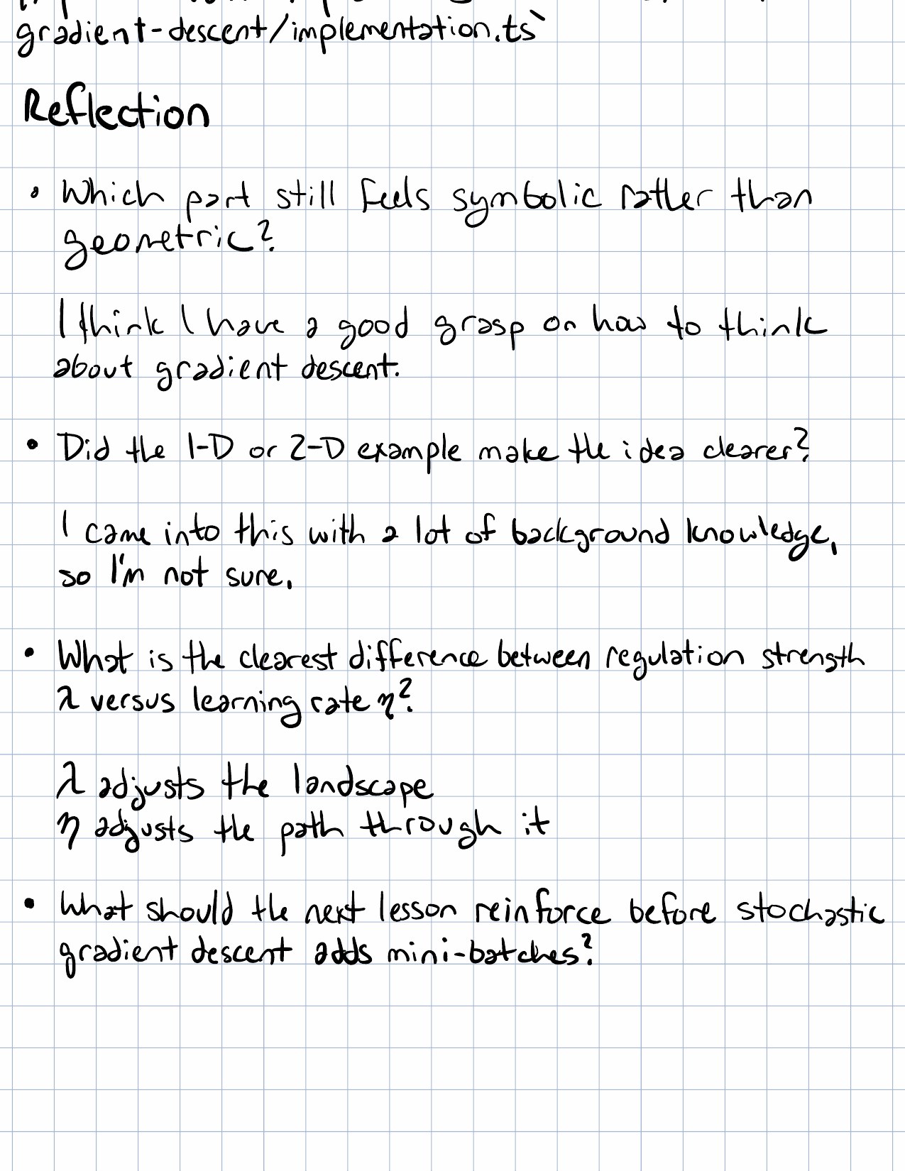
Which part of the update rule carries the “downhill” meaning?
What changes when the loss is multiplied by 100?
How is early stopping different from gradient descent itself?
Why might a long, narrow loss valley make optimization difficult?
Which symbols were easiest to remember, and which ones still need a local table?

Next Lesson

Next: Stochastic Gradient Descent.

The bridge is simple: full gradient descent uses the whole dataset to compute the gradient, while stochastic gradient descent uses one example or a mini-batch to estimate the gradient more cheaply and more noisily.

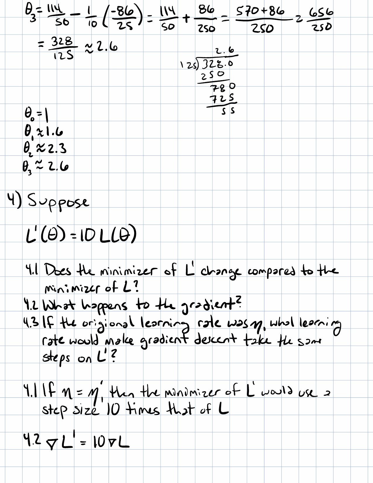
Completed Exercises

Handwritten work submitted after completing this lesson.