Lesson 27: Stochastic Gradient Descent

Goal

Understand stochastic gradient descent as the practical version of gradient descent used for large machine learning problems: instead of computing the exact gradient from the whole dataset before every update, estimate that gradient from one example or a small mini-batch.

The core tradeoff is:

Full gradient descent gives a clean direction slowly. Stochastic gradient descent gives a noisy direction quickly.

Review: full gradient descent

In full gradient descent, the loss over the dataset is the average loss over all examples:

J(θ) = \frac{1}{N}\sum_{i=1}^{N} L_i(θ)

where:

N is the number of training examples.
θ is the vector of model parameters.
L_i(θ) is the loss from example i.
J(θ) is the average dataset loss.

The gradient is also an average:

∇J(θ) = \frac{1}{N}\sum_{i=1}^{N} ∇L_i(θ)

Then the update rule is:

θ \leftarrow θ - η∇J(θ)

This is conceptually clean, but expensive. One update requires looking at every training example.

Why full gradient descent becomes impractical

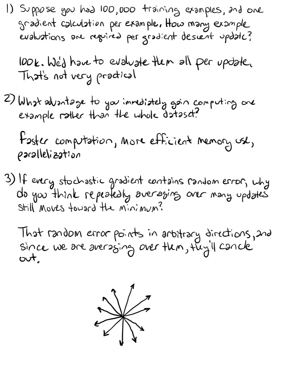
Suppose we have 100,000 training examples and need one gradient computation per example.

One full gradient descent update requires 100,000 example evaluations.

That is fine for a toy problem. It is not fine for millions or billions of examples, especially when each example flows through a large neural network.

The problem is not that full gradient descent is mathematically wrong. The problem is that exactness is too expensive.

The stochastic idea

Instead of computing the full average gradient,

∇J(θ) = \frac{1}{N}\sum_{i=1}^{N} ∇L_i(θ)

choose one random example j and use its gradient:

∇L_j(θ)

Then update:

θ \leftarrow θ - η∇L_j(θ)

This is stochastic gradient descent, or SGD.

The word stochastic means random. The randomness comes from choosing a random training example or random mini-batch.

Why this does not immediately fail

A single example may point in a noisy direction. It may point too far left, too far right, or with the wrong magnitude.

But if examples are sampled randomly, the expected stochastic gradient equals the full gradient:

E[∇L_i(θ)] = ∇J(θ)

where E[·] means expected value.

This makes the stochastic gradient an unbiased estimator of the full gradient.

That does not mean every individual step is correct. It means the errors do not systematically point in the wrong direction. Over many updates, the random errors tend to cancel.

The zig-zag path

Full gradient descent tends to follow a smoother path because every update uses the full dataset.

SGD tends to zig-zag because each update uses only a noisy estimate of the full gradient.

The important distinction:

Full gradient descent moves slowly but smoothly.
SGD moves quickly but noisily.

The noisy path is not a bug. It is part of why SGD is useful.

Noise and sharp minima

A sharp minimum is a narrow valley in the loss landscape. A flat minimum is a wider valley.

Gradient noise can bump the parameters around. Those bumps can knock the optimizer out of narrow valleys more easily than wide valleys.

This matters because flat minima are often more robust: small changes to the parameters do not change the loss very much. That robustness is one reason flat minima are often associated with better generalization.

So the noise in SGD can be useful. It can make optimization less likely to settle into a fragile solution.

Mini-batch gradient descent

In practice, neural networks usually do not use a single example per update.

Instead, they use a mini-batch: a small random subset of the training data.

Common batch sizes include 16, 32, 64, 128, 256, or 512, though the right value depends on the model, data, and hardware.

For a mini-batch of size m, the gradient estimate is:

∇J(θ) \approx \frac{1}{m}\sum_{i=1}^{m} ∇L_i(θ)

where m is the batch size.

Mini-batches are a compromise:

They are much cheaper than the full dataset.
They are less noisy than a single example.
They use GPUs more efficiently than a single example.
They make updates more stable.

Today, when people say “SGD,” they often mean mini-batch SGD.

Batch size tradeoffs

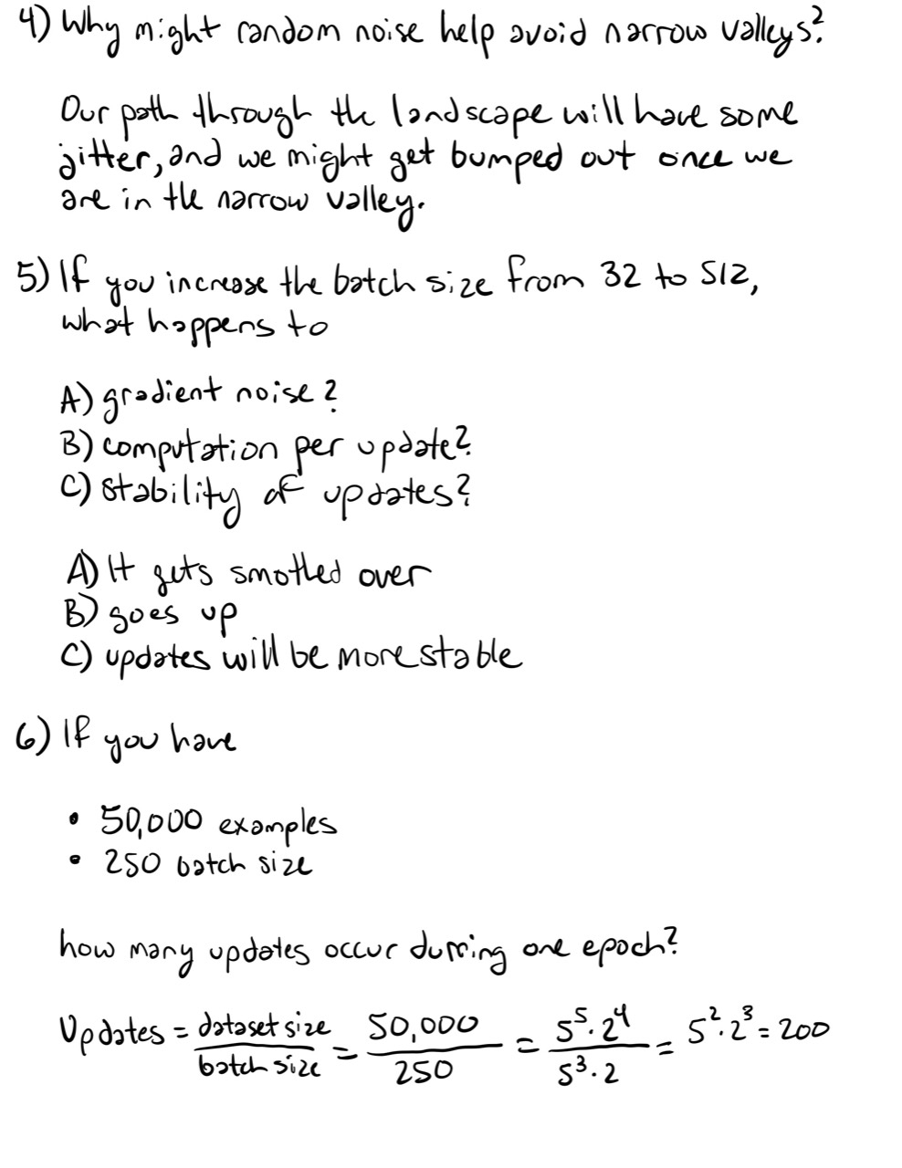
Increasing batch size usually does three things:

Decreases gradient noise.
Increases computation per update.
Makes each update more stable.

But larger batches also use more memory and produce fewer updates per epoch.

Smaller batches are noisier but can update more frequently. They may also generalize better in some settings because the noise acts like a weak regularizer.

Epochs

An epoch is one complete pass through the training dataset.

If:

N is the dataset size
m is the batch size

then the number of updates per epoch is:

\text{updates per epoch} = \frac{N}{m}

For example, with 50,000 examples and batch size 250:

\frac{50,000}{250} = 200

So one epoch contains 200 updates.

With 120,000 examples and batch size 240:

\frac{120,000}{240} = 500

So one epoch contains 500 updates.

Shuffling

Before each epoch, the dataset is usually shuffled.

This prevents the optimizer from learning artifacts of the data order. For example, without shuffling, a model might see many examples from the same class in a row, causing mini-batches to be poor representatives of the whole dataset.

Shuffling makes each mini-batch closer to a random sample of the dataset.

Practical consequences

If GPU memory doubles, a few things become possible:

Increase batch size.
Train a larger model.
Use larger inputs, such as higher-resolution images.
Use longer sequences in language or time-series models.

The most direct SGD-related consequence is that a larger batch size becomes possible.

Summary

Stochastic gradient descent replaces exact gradients with random estimates.

Full gradient descent computes:

∇J(θ) = \frac{1}{N}\sum_{i=1}^{N} ∇L_i(θ)

SGD estimates that direction using one example or a mini-batch.

The estimate is noisy but, under random sampling, unbiased:

E[∇L_i(θ)] = ∇J(θ)

The noise causes zig-zag motion, but it can also help optimization avoid sharp minima. Mini-batches balance speed, stability, hardware efficiency, and noise.

Common arithmetic checks

Two common update-per-epoch calculations:

\frac{50,000}{250} = 200

\frac{120,000}{240} = 500

When the formula is right but the number is wrong, treat that as an arithmetic slip, not a conceptual error.

Exercises

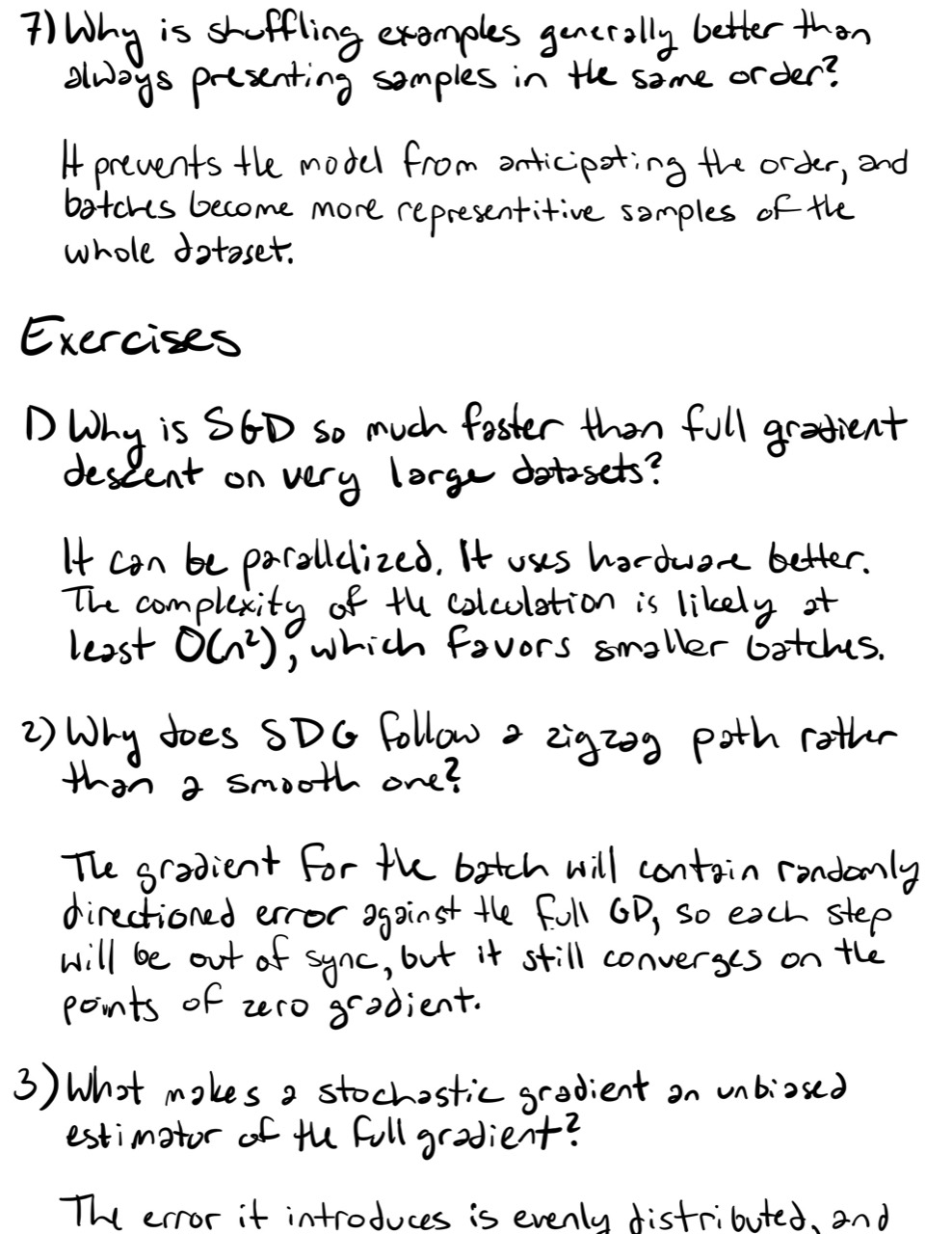
Explain why SGD is much faster than full gradient descent on very large datasets.
Why does SGD follow a zig-zag path instead of a smooth one?
What makes a stochastic gradient an unbiased estimator of the full gradient?
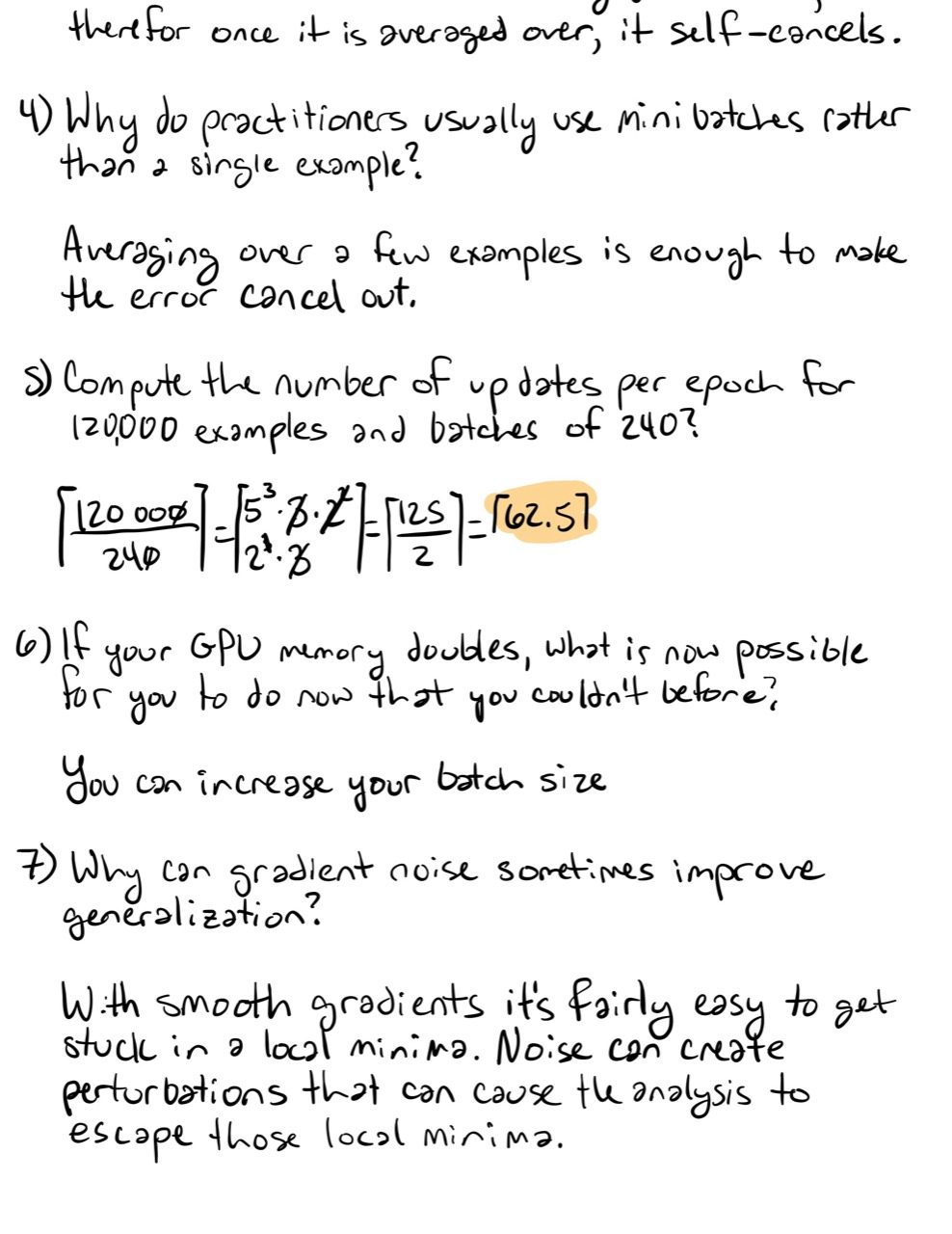
Why do practitioners usually use mini-batches instead of a single example?
Compute the number of updates per epoch for:
- Dataset: 120,000 examples
- Batch size: 240
If GPU memory doubles, what practical change to training becomes possible?
In your own words, explain why gradient noise can sometimes improve generalization.

Looking ahead

SGD gives us fast but noisy updates.

The next question is:

Can we keep the speed of SGD while reducing useless oscillation?

That leads to momentum, where the optimizer remembers previous update directions and accumulates velocity through the loss landscape.

Completed Exercises

Handwritten work submitted after completing this lesson.