Lesson 28: Momentum | Mathematics of AI

Goal

Understand momentum as a small modification to stochastic gradient descent: instead of choosing each update direction only from the current noisy gradient, keep a velocity vector that remembers recent directions.

The core idea is:

SGD asks, “Which way is downhill right now?” Momentum asks, “Which way have we consistently been going downhill?”

Review: SGD

In mini-batch stochastic gradient descent, we estimate the gradient from a batch of training examples:

g_t \approx \nabla J(\theta_t)

Then we update parameters with:

\theta_{t+1} = \theta_t - \eta g_t

where:

θ_t is the current parameter vector.
g_t is the gradient estimate at step t.
η is the learning rate.

This works, but g_t is noisy. Each batch gives a slightly different direction.

The zig-zag problem

Imagine the loss landscape has a long, narrow valley.

One direction points across the valley wall. Another direction points along the valley toward lower loss.

SGD often sees gradients that bounce from one wall to the other:

left wall -> right wall -> left wall -> right wall

That means many updates cancel each other sideways. The optimizer is technically moving downhill, but part of the motion is wasted as oscillation.

The useful direction is the one that keeps recurring across many steps.

Momentum tries to preserve that persistent direction and dampen the back-and-forth direction.

The physical metaphor

Plain SGD behaves like a marble that forgets its previous motion after every step.

Momentum behaves more like a ball with inertia:

If the slope keeps pointing in roughly the same direction, the ball speeds up.
If the slope alternates left and right, those sideways pushes cancel.
If the direction changes, the ball does not instantly turn; it carries some previous velocity.

This is only a metaphor, but it is a useful one. Momentum gives the optimizer memory.

Velocity

Momentum introduces a new vector, v_t, called the velocity.

The velocity is not the model parameter. It is the optimizer’s remembered update direction.

A common momentum update is:

v_t = \beta v_{t-1} + g_t

Then parameters are updated with:

\theta_{t+1} = \theta_t - \eta v_t

where:

v_t is the current velocity.
v_{t-1} is the previous velocity.
g_t is the current gradient estimate.
β is the momentum coefficient.
η is the learning rate.

The term β v_{t-1} keeps part of the previous velocity. The term g_t adds the current gradient.

What beta does

The momentum coefficient β controls memory.

If β = 0, then:

v_t = g_t

and the update becomes ordinary SGD:

\theta_{t+1} = \theta_t - \eta g_t

If β is close to 1, the optimizer keeps a lot of previous velocity.

Common values include:

β = 0.9

That means the new velocity keeps 90% of the previous velocity and adds the current gradient.

Do not read β = 0.9 as “ignore the current gradient.” The current gradient is still added. The point is that recent history matters.

Learning rate versus momentum

The learning rate η and momentum coefficient β do different jobs.

η controls how large the parameter update is:

\theta_{t+1} = \theta_t - \eta v_t

β controls how much previous velocity survives:

v_t = \beta v_{t-1} + g_t

A useful programming analogy:

g_t is the latest input signal.
v_t is state stored by the optimizer.
β controls how much old state persists.
η controls how strongly the state changes the model parameters.

Why momentum reduces zig-zagging

Suppose the sideways component of the gradient alternates:

step 1: push left
step 2: push right
step 3: push left
step 4: push right

Those components partially cancel in the velocity because they do not persist.

Now suppose the downhill-along-the-valley component keeps pointing forward:

step 1: push forward
step 2: push forward
step 3: push forward
step 4: push forward

Those components accumulate in the velocity.

So momentum tends to:

reduce oscillation across narrow valleys;
increase speed along consistent downhill directions;
smooth noisy mini-batch gradients;
make optimization less myopic.

A one-dimensional example

Suppose the previous velocity is:

v_{t-1} = 4

The current gradient is:

g_t = 3

and:

\beta = 0.9

Then:

v_t = 0.9(4) + 3 = 3.6 + 3 = 6.6

If the learning rate is:

\eta = 0.1

then the parameter update is:

\theta_{t+1} = \theta_t - 0.1(6.6)

so:

\theta_{t+1} = \theta_t - 0.66

The update is larger than the current gradient alone would have produced because the previous direction agreed with the current direction.

A cancellation example

Now suppose the previous velocity is:

v_{t-1} = 4

but the current gradient points the other way:

g_t = -3

With β = 0.9:

v_t = 0.9(4) + (-3) = 3.6 - 3 = 0.6

The new velocity is much smaller. The optimizer does not fully reverse direction immediately, but the opposing gradient slows it down.

That is the damping behavior we want when noisy gradients alternate.

Momentum as exponential memory

The velocity contains a weighted history of past gradients.

Expanding the recurrence:

v_t = \beta v_{t-1} + g_t

and substituting for v_{t-1} gives:

v_t = g_t + \beta g_{t-1} + \beta^2 g_{t-2} + \beta^3 g_{t-3} + \cdots

Recent gradients matter more. Older gradients still matter, but their influence decays by powers of β.

This is why momentum is a kind of exponentially weighted memory.

Connection to programming

In plain SGD, the optimizer update can be written as a stateless function of the current gradient:

new_theta = theta - learning_rate * gradient

With momentum, the optimizer has state:

velocity = beta * velocity + gradient
new_theta = theta - learning_rate * velocity

So momentum is not a new model. It is a new optimizer state variable.

The model still stores parameters. The optimizer stores velocity.

Common variants

Different texts write momentum with slightly different conventions.

One common version is:

v_t = \beta v_{t-1} + g_t

\theta_{t+1} = \theta_t - \eta v_t

Another common version folds the learning rate into the velocity:

v_t = \beta v_{t-1} - \eta g_t

\theta_{t+1} = \theta_t + v_t

These are not conceptually different. They package the same idea in different variables.

When reading papers or documentation, always check where the minus sign and learning rate are placed.

What momentum does not solve

Momentum does not magically pick the perfect learning rate.

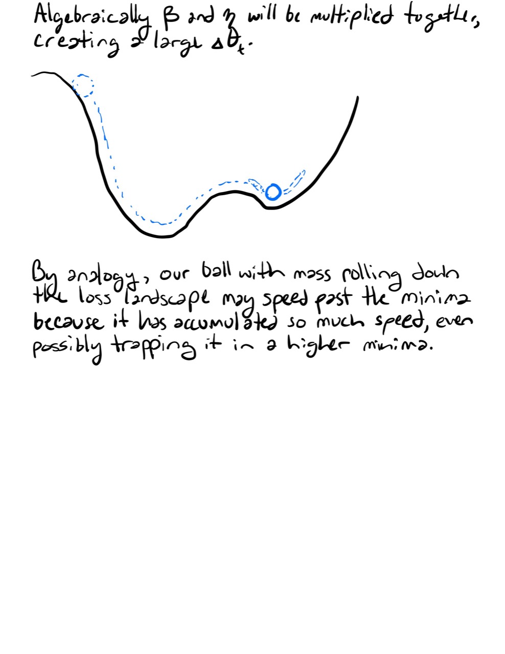
If the learning rate is too large, momentum can make instability worse because velocity may build up too much.

Momentum also does not remove gradient noise completely. It smooths it.

The practical lesson:

Momentum helps when recent gradients contain a real persistent direction, but it can overshoot when the optimizer accumulates too much velocity.

Summary

SGD uses the current gradient estimate:

\theta_{t+1} = \theta_t - \eta g_t

Momentum adds velocity:

v_t = \beta v_{t-1} + g_t

\theta_{t+1} = \theta_t - \eta v_t

The velocity remembers recent gradient directions. Directions that persist accumulate. Directions that alternate tend to cancel.

This makes momentum useful for reducing zig-zagging, smoothing noisy SGD updates, and moving faster through long valleys in the loss landscape.

Exercises

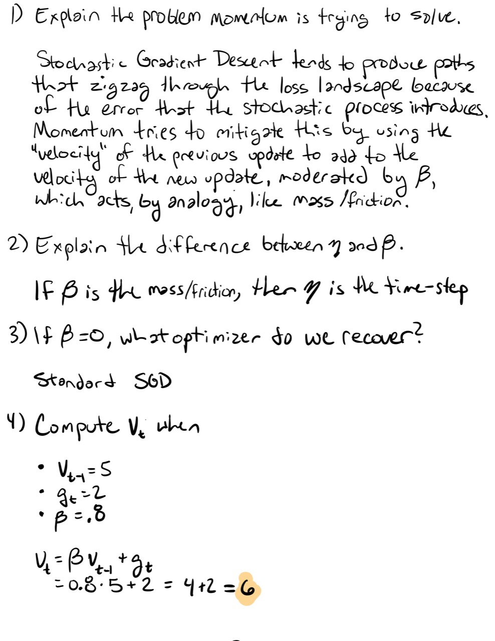
In your own words, explain what problem momentum is trying to solve.
What is the difference between η and β?
If β = 0, what optimizer do we recover?
Compute v_t when:
- v_{t-1} = 5
- g_t = 2
- β = 0.8
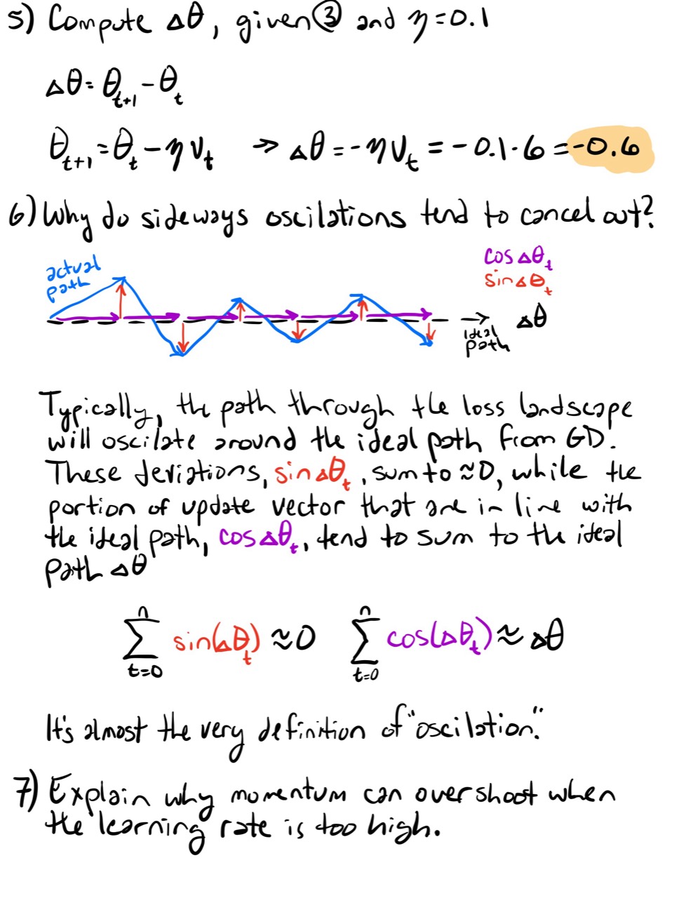
Compute the parameter update if η = 0.1 and the velocity from exercise 4 is used.
Why do sideways oscillations tend to cancel under momentum?
Explain why momentum can overshoot if the learning rate is too large.

Looking ahead

Momentum remembers recent gradient directions, but it uses one shared learning rate scale for all parameters.

The next question is:

Can an optimizer adapt the update size separately for different parameters?

That leads to adaptive optimizers such as Adam, which combines momentum-like memory with per-parameter scaling.

Completed Exercises

Handwritten work submitted after completing this lesson.