Lesson 29: Adam | Mathematics of AI

Goal

Understand Adam as an adaptive optimizer that keeps two memories:

a momentum-like memory of recent gradients;
a scale memory of recent squared gradients.

The core idea is:

Adam asks, “Which direction has been consistently useful, and how large are gradients usually in each parameter?”

By the end of the lesson, Adam should feel less like a magic optimizer name and more like a stateful update rule built from ideas you already know: SGD, momentum, exponential memory, and per-parameter scaling.

Motivation

Gradient descent gave us the basic movement rule:

\theta_{t+1} = \theta_t - \eta \nabla L(\theta_t)

SGD made that rule practical by estimating the gradient from mini-batches:

\theta_{t+1} = \theta_t - \eta g_t

Momentum added memory:

v_t = \beta v_{t-1} + g_t

\theta_{t+1} = \theta_t - \eta v_t

That helps when the same downhill direction keeps recurring.

But momentum still uses one shared learning-rate scale. If one parameter usually has huge gradients and another usually has tiny gradients, a single global step size can be awkward:

The large-gradient parameter may move too aggressively.
The small-gradient parameter may move too slowly.
A learning rate that is safe for one coordinate may be inefficient for another.

Adam responds by adapting the update size separately for each parameter.

Prerequisites

Lesson 26: Gradient Descent.
Lesson 27: Stochastic Gradient Descent.
Lesson 28: Momentum.
Comfort reading elementwise vector operations.

Notation / Symbol Table

Symbol	Plain-English name	Meaning
$\theta_t$	current parameters	The parameter vector at optimization step $t$ .
$g_t$	gradient estimate	The mini-batch gradient estimate at step $t$ .
$m_t$	first moment estimate	A running average of recent gradients.
$v_t$	second moment estimate	A running average of recent squared gradients.
$\hat{m}_t$	bias-corrected first moment	$m_t$ adjusted for zero initialization.
$\hat{v}_t$	bias-corrected second moment	$v_t$ adjusted for zero initialization.
$\beta_1$	first-moment decay	How much previous gradient memory is retained.
$\beta_2$	second-moment decay	How much previous squared-gradient memory is retained.
$\eta$	base learning rate	The global scale applied to Adam’s normalized update.
$\epsilon$	stability constant	Small positive number added to avoid division by zero.
$\odot$	elementwise multiplication	Multiply matching coordinates separately.

Important overload warning: in Lesson 28, $v_t$ meant momentum velocity. In Adam, $v_t$ usually means the second moment estimate. Same letter, different optimizer state. Always check the local symbol table.

Core Idea

Adam is short for adaptive moment estimation.

The name is useful once the vocabulary is unpacked:

Adaptive means different parameters can get different effective step sizes.
Moment means a summary of a distribution or sequence.
The first moment is like an average value.
The second raw moment is like an average squared value.

For Adam, the sequence being summarized is the sequence of mini-batch gradients.

The first memory tracks the average gradient direction. The second memory tracks the average squared gradient size.

First Memory: Direction

Adam’s first memory is:

m_t = \beta_1 m_{t-1} + (1 - \beta_1)g_t

This looks like momentum. It keeps a running average of recent gradients.

If recent gradients keep pointing in the same direction, $m_t$ keeps that direction. If gradients alternate, the running average dampens the noise.

The coefficient $\beta_1$ controls how much previous first-moment memory survives. A common default is:

beta_1 = 0.9

That means the new first moment keeps 90 percent of the previous first moment and blends in 10 percent of the current gradient.

Second Memory: Scale

Adam’s second memory is:

v_t = \beta_2 v_{t-1} + (1 - \beta_2)(g_t \odot g_t)

The term $g_t \odot g_t$ means square each gradient coordinate separately.

If:

g_t = [10, 1]

then:

g_t \odot g_t = [100, 1]

So $v_t$ tracks which coordinates usually have large gradients and which usually have small gradients.

A common default is:

beta_2 = 0.999

That makes the second memory change slowly. It is trying to estimate a stable scale for each parameter, not react sharply to one noisy mini-batch.

Why Squared Gradients Help

Suppose two parameters have different gradient scales:

g_t = [10, 1]

Plain SGD uses the same learning rate for both coordinates:

\Delta \theta = -\eta [10, 1]

The first coordinate moves ten times as much as the second.

Adam divides by a running estimate of gradient scale:

\frac{\hat{m}_t}{\sqrt{\hat{v}_t} + \epsilon}

The square root matters because $v_t$ stores squared gradients. If a coordinate has squared-gradient scale near 100, then $\sqrt{100} = 10$ .

Very roughly:

\frac{[10, 1]}{\sqrt{[100, 1]}} = \frac{[10, 1]}{[10, 1]} = [1, 1]

This is the adaptive part. Adam reduces updates in coordinates that usually have large gradients and allows relatively larger updates in coordinates that usually have small gradients.

Bias Correction

Adam usually initializes both memories at zero:

m_0 = 0

v_0 = 0

Early in training, that makes the running averages biased toward zero. For example:

m_1 = \beta_1 m_0 + (1 - \beta_1)g_1

Since $m_0 = 0$ :

m_1 = (1 - \beta_1)g_1

If $\beta_1 = 0.9$ , then $m_1$ is only 10 percent of $g_1$ .

Adam corrects this with:

\hat{m}_t = \frac{m_t}{1 - \beta_1^t}

and:

\hat{v}_t = \frac{v_t}{1 - \beta_2^t}

The hats mean “bias-corrected.” They compensate for the fact that the memories started at zero.

The Adam Update Rule

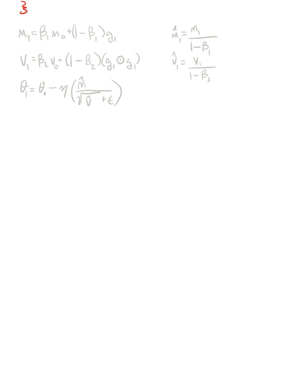
Adam computes:

m_t = \beta_1 m_{t-1} + (1 - \beta_1)g_t

v_t = \beta_2 v_{t-1} + (1 - \beta_2)(g_t \odot g_t)

Then it bias-corrects:

\hat{m}_t = \frac{m_t}{1 - \beta_1^t}

\hat{v}_t = \frac{v_t}{1 - \beta_2^t}

Finally it updates:

\theta_{t+1} = \theta_t - \eta \frac{\hat{m}_t}{\sqrt{\hat{v}_t} + \epsilon}

Read the last line as:

Move opposite the momentum-like average gradient, scaled coordinate-by-coordinate by recent gradient magnitude.

The division is elementwise. Each parameter gets its own denominator.

A Small Scalar Example

Use toy coefficients to keep the arithmetic small:

beta_1 = 0.8
beta_2 = 0.9
eta = 0.1
epsilon is tiny enough to ignore

Start with:

m_0 = 0

v_0 = 0

and suppose:

g_1 = 3

First moment:

m_1 = 0.8(0) + (1 - 0.8)(3) = 0.6

Second moment:

v_1 = 0.9(0) + (1 - 0.9)(3^2) = 0.9

Bias correction:

\hat{m}_1 = \frac{0.6}{1 - 0.8^1} = \frac{0.6}{0.2} = 3

\hat{v}_1 = \frac{0.9}{1 - 0.9^1} = \frac{0.9}{0.1} = 9

Adam update:

\theta_2 = \theta_1 - 0.1 \frac{3}{\sqrt{9} + \epsilon}

Ignoring the tiny $\epsilon$ :

\theta_2 \approx \theta_1 - 0.1

This example shows a useful first-step behavior: after bias correction, Adam has recovered the gradient scale information from the first observation.

Connection To RMSProp

You will often see Adam described as combining momentum and RMSProp.

RMSProp keeps a running average of squared gradients and divides by the root mean square scale:

s_t = \rho s_{t-1} + (1 - \rho)(g_t \odot g_t)

\theta_{t+1} = \theta_t - \eta \frac{g_t}{\sqrt{s_t} + \epsilon}

Adam adds the momentum-like first moment $m_t$ and bias correction:

\theta_{t+1} = \theta_t - \eta \frac{\hat{m}_t}{\sqrt{\hat{v}_t} + \epsilon}

That is the conceptual compression:

Adam is momentum for direction plus RMSProp-style scaling for step size.

Connection To Programming

Plain SGD needs almost no optimizer state:

theta = theta - learning_rate * gradient

Momentum stores one state vector:

velocity = beta * velocity + gradient
theta = theta - learning_rate * velocity

Adam stores two state vectors:

firstMoment = beta1 * firstMoment + (1 - beta1) * gradient
secondMoment = beta2 * secondMoment + (1 - beta2) * gradient * gradient
firstMomentHat = firstMoment / (1 - beta1 ** step)
secondMomentHat = secondMoment / (1 - beta2 ** step)
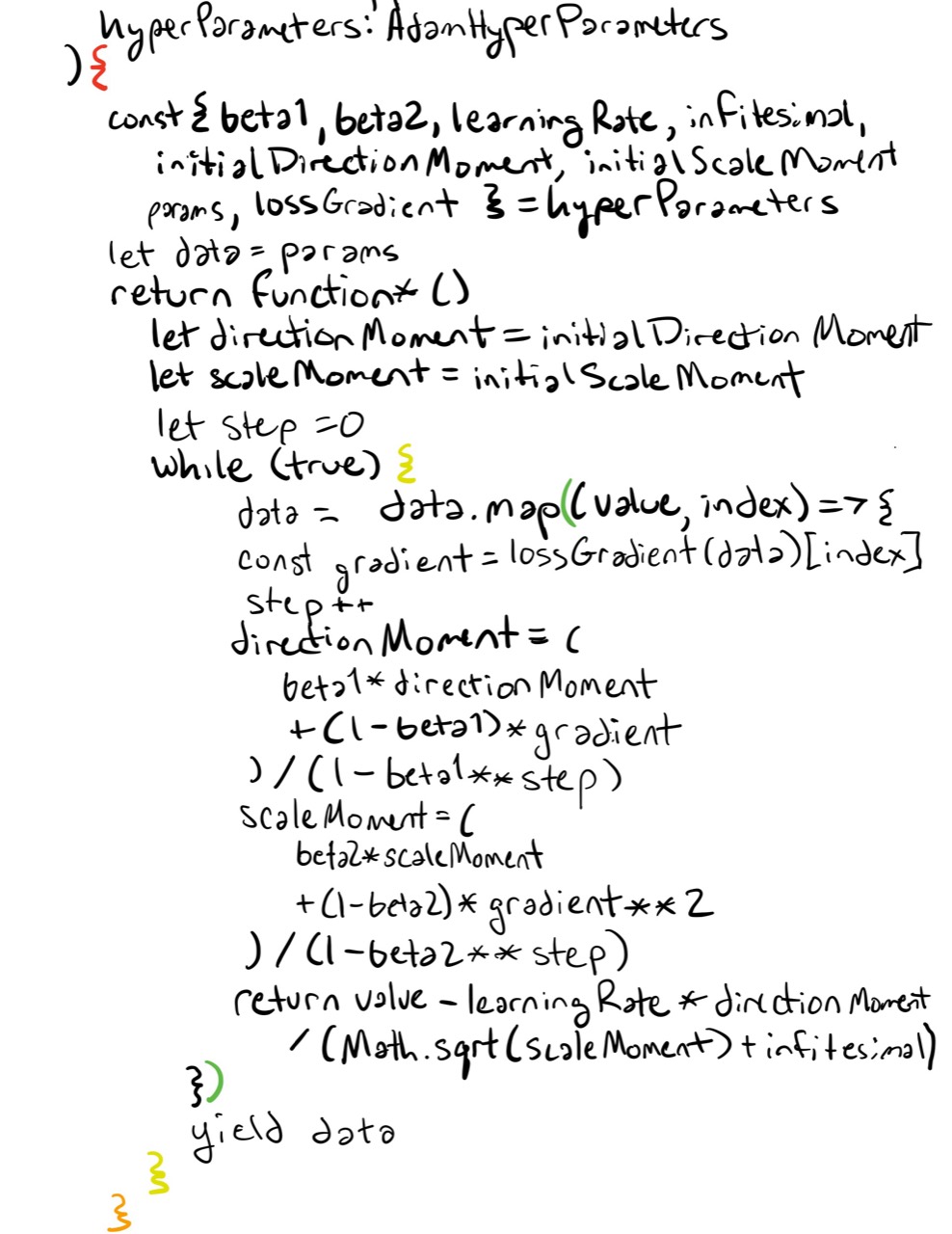
theta = theta - learningRate * firstMomentHat / (sqrt(secondMomentHat) + epsilon)

The model stores parameters. The optimizer stores memory about gradients.

What Adam Helps With

Adam is often useful when:

gradients are noisy;
different parameters have very different gradient scales;
sparse features cause some parameters to receive updates rarely;
a model needs a strong practical default before careful tuning.

That is why Adam is common in deep learning experiments. It often starts training effectively without as much learning-rate tuning as plain SGD.

What Adam Does Not Solve

Adam is not a guarantee of better generalization.

It can make optimization easier, but it does not replace:

choosing a good model;
choosing a good loss;
using appropriate regularization;
checking validation behavior;
tuning the learning rate;
understanding weight decay.

One important warning for later: weight decay interacts differently with adaptive optimizers than with plain SGD. This is why AdamW exists. AdamW is not the topic yet, but the warning is worth naming so “Adam plus weight decay” does not become a blurry phrase.

Why Adam Shows Up In ML

Modern neural networks often have many parameters with very different roles and gradient scales.

For example:

embeddings may update sparsely;
normalization parameters may have different scales from dense-layer weights;
attention projections may see different gradient patterns from feed-forward layers;
mini-batch noise may vary across training.

Adam gives each parameter a local scale estimate while still using a momentum-like direction estimate. That makes it a strong default optimizer for many experiments.

Summary

SGD uses the current gradient estimate:

\theta_{t+1} = \theta_t - \eta g_t

Momentum remembers recent gradient directions:

v_t = \beta v_{t-1} + g_t

Adam keeps two memories:

m_t = \beta_1 m_{t-1} + (1 - \beta_1)g_t

v_t = \beta_2 v_{t-1} + (1 - \beta_2)(g_t \odot g_t)

Then Adam updates with:

\theta_{t+1} = \theta_t - \eta \frac{\hat{m}_t}{\sqrt{\hat{v}_t} + \epsilon}

The first moment gives direction. The second moment gives scale. Bias correction fixes the early zero-initialization shrinkage.

Exercises

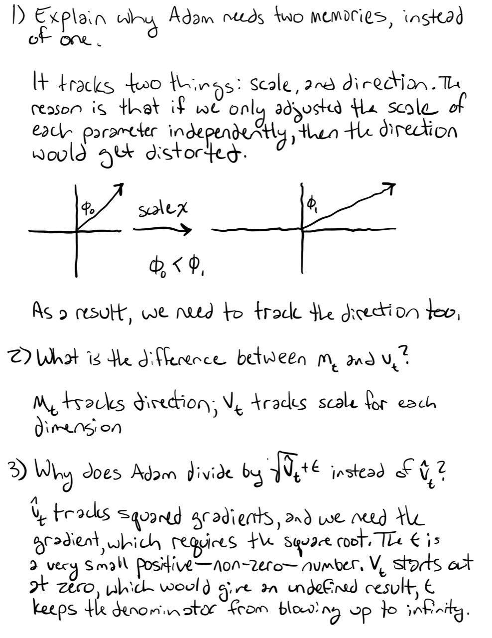
In your own words, explain why Adam needs two memories instead of one.
What is the difference between $m_t$ and $v_t$ in Adam?
Why does Adam divide by $\sqrt{\hat{v}_t} + \epsilon$ instead of by $\hat{v}_t$ ?
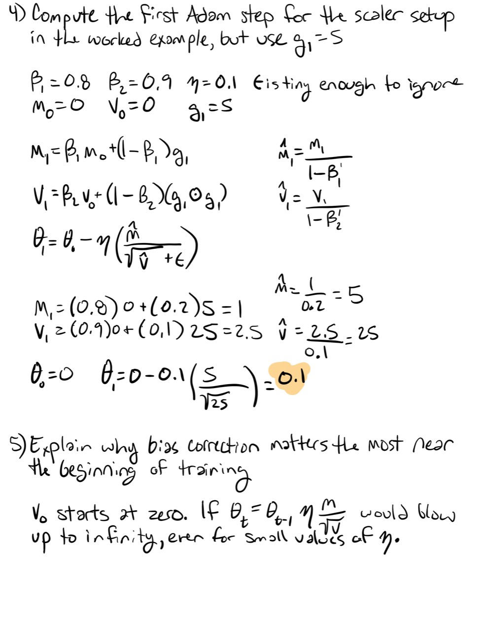
Compute the first Adam step for the scalar setup in the worked example, but use $g_1 = 5$ .
Explain why bias correction matters most near the beginning of training.
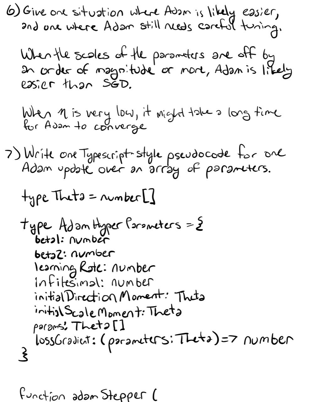
Give one situation where Adam is likely easier to use than plain SGD, and one situation where Adam still needs careful tuning.
Write TypeScript-style pseudocode for one Adam update over an array of parameters.

Looking Ahead

Adam adapts step sizes using gradient history, but it still has a base learning rate $\eta$ .

The next question is:

Should the base learning rate itself change over training?

That leads to learning rate schedules: decay, warmup, cosine schedules, and the practical shape of training runs.

Completed Exercises

Handwritten work submitted after completing this lesson.