Lesson 30: Learning Rate Schedules

Goal

Understand learning rate schedules as a way to change the optimizer’s base step size over time.

The core idea is:

Early training often needs exploration and fast progress. Late training often needs smaller, more careful steps.

A learning rate schedule turns the learning rate from a constant into a function:

\eta_t = f(t)

The optimizer still decides the update direction. The schedule decides how large the base step should be at step $t$ .

Motivation

Gradient descent used a fixed learning rate:

\theta_{t+1} = \theta_t - \eta \nabla L(\theta_t)

SGD used a noisy gradient estimate:

\theta_{t+1} = \theta_t - \eta g_t

Momentum and Adam added optimizer state, but they still usually have a base learning rate.

A fixed learning rate asks one number to serve the whole training run:

large enough to move quickly at the beginning;
small enough not to bounce around near the end;
safe enough for unstable early gradients;
useful enough after the model has mostly learned the easy structure.

That is a lot to ask from one scalar.

A schedule says: use different step sizes at different phases of training.

Prerequisites

Lesson 26: Gradient Descent.
Lesson 27: Stochastic Gradient Descent.
Lesson 28: Momentum.
Lesson 29: Adam.
Comfort reading simple piecewise functions.

Notation / Symbol Table

Symbol	Plain-English name	Meaning
$\eta$	learning rate	Base step size.
$\eta_t$	scheduled learning rate	Learning rate at step $t$ .
$t$	step	Current optimizer step.
$T$	total steps	Total planned schedule length.
$T_w$	warmup steps	Number of early steps spent increasing the learning rate.
$\eta_{max}$	maximum learning rate	Target or peak learning rate.
$\eta_{min}$	minimum learning rate	Floor learning rate near the end.
$f(t)$	schedule function	Function that maps step number to learning rate.

The Schedule Is Outside The Gradient

With SGD, a schedule changes:

\theta_{t+1} = \theta_t - \eta g_t

into:

\theta_{t+1} = \theta_t - \eta_t g_t

The gradient $g_t$ says which direction looks downhill from the current mini-batch.

The learning rate $\eta_t$ says how far to move in that direction.

For Adam, the update becomes:

\theta_{t+1} = \theta_t - \eta_t \frac{\hat{m}_t}{\sqrt{\hat{v}_t} + \epsilon}

Adam adapts coordinate-by-coordinate using optimizer memory. The schedule still scales the whole Adam update at step $t$ .

Mental Model: Three Training Phases

A useful rough model is:

Phase	What is happening	Learning-rate need
Early	Parameters are poorly placed; gradients may be unstable.	Sometimes ramp up gradually.
Middle	Model is finding broad useful structure.	Often use the largest effective learning rate.
Late	Model is refining.	Often decay to smaller steps.

This is not a theorem. It is an engineering pattern that shows up because optimization behavior changes during training.

Constant Learning Rate

The simplest schedule is no schedule:

\eta_t = \eta

This can work, especially for simple problems.

Its weakness is that it gives the same step scale to early, middle, and late training.

Step Decay

Step decay keeps the learning rate constant for a while, then drops it sharply.

Example:

\eta_t = \begin{cases} 0.1 & t < 1000 \\ 0.01 & 1000 \le t < 2000 \\ 0.001 & t \ge 2000 \end{cases}

Read this as:

Train aggressively first, then reduce the step size at known milestones.

Step decay is easy to reason about, but the drop points are hand-chosen.

Exponential Decay

Exponential decay shrinks the learning rate smoothly by multiplying by a decay factor:

\eta_t = \eta_0 \gamma^t

where:

$\eta_0$ is the initial learning rate;
$\gamma$ is a decay factor, usually slightly less than 1.

If $\gamma = 0.99$ , then each step keeps 99 percent of the previous learning rate.

This is exponential memory again: the same shape you saw in momentum and Adam, but applied to the learning rate itself.

Linear Decay

Linear decay moves from a maximum learning rate to a minimum learning rate in a straight line:

\eta_t = \eta_{max} - \frac{t}{T}(\eta_{max} - \eta_{min})

At $t = 0$ :

\eta_0 = \eta_{max}

At $t = T$ :

\eta_T = \eta_{min}

This is easy to implement and easy to inspect.

Warmup

Warmup starts with a small learning rate and increases it over the first $T_w$ steps.

A simple linear warmup is:

\eta_t = \eta_{max} \frac{t}{T_w}

for:

0 \le t \le T_w

So if $T_w = 1000$ , then step 500 uses about half the target learning rate.

Warmup is common with large neural networks because the earliest gradients can be poorly scaled. Starting too aggressively can damage training before the optimizer state has useful information.

For Adam, this is especially intuitive: Adam’s first and second moment estimates are still forming at the beginning.

Warmup Plus Decay

A common pattern is:

warm up from a small learning rate to $\eta_{max}$ ;
decay from $\eta_{max}$ toward $\eta_{min}$ .

This gives the schedule a shape like:

small -> larger -> smaller

That may look odd at first. Why not start large immediately?

Because early training is not just “far from the minimum.” It is also poorly calibrated. The optimizer has not yet built useful state, and the model’s activations and gradients may be unstable.

Cosine Decay

Cosine decay is a smooth decay that starts flat, falls more sharply in the middle, and flattens again near the end.

One common form is:

\eta_t = \eta_{min} + \frac{1}{2}(\eta_{max} - \eta_{min})\left(1 + \cos\left(\pi \frac{t}{T}\right)\right)

Check the endpoints.

At $t = 0$ :

\cos(0) = 1

so:

\eta_0 = \eta_{max}

At $t = T$ :

\cos(\pi) = -1

so:

\eta_T = \eta_{min}

The cosine is not magic. It is a convenient smooth curve with gentle endpoints.

Worked Example: Linear Warmup

Suppose:

eta_max = 0.001
warmup_steps = 1000

Use:

\eta_t = \eta_{max}\frac{t}{T_w}

At step 250:

\eta_{250} = 0.001 \cdot \frac{250}{1000} = 0.00025

At step 500:

\eta_{500} = 0.001 \cdot \frac{500}{1000} = 0.0005

At step 1000:

\eta_{1000} = 0.001 \cdot \frac{1000}{1000} = 0.001

The schedule is not changing the gradient. It is changing how much trust the optimizer puts in the update at that step.

Worked Example: Step Decay

Suppose:

initial learning rate = 0.1
drop every 1000 steps
multiply by 0.1 at each drop

Then:

Step range	Learning rate
0 to 999	0.1
1000 to 1999	0.01
2000 to 2999	0.001

This kind of schedule is simple and explicit. The cost is that the boundaries are discontinuous.

Connection To Programming

A schedule is just a function.

function constantLearningRate(step: number): number {
  return 0.001;
}

Linear warmup:

function linearWarmup(step: number, warmupSteps: number, maxLearningRate: number): number {
  const fraction = Math.min(step / warmupSteps, 1);
  return maxLearningRate * fraction;
}

Cosine decay:

function cosineDecay(
  step: number,
  totalSteps: number,
  maxLearningRate: number,
  minLearningRate: number,
): number {
  const progress = Math.min(step / totalSteps, 1);
  return minLearningRate + 0.5 * (maxLearningRate - minLearningRate) *
    (1 + Math.cos(Math.PI * progress));
}

Warmup followed by cosine decay:

function warmupThenCosine(
  step: number,
  warmupSteps: number,
  totalSteps: number,
  maxLearningRate: number,
  minLearningRate: number,
): number {
  if (step < warmupSteps) {
    return maxLearningRate * (step / warmupSteps);
  }

  const decayStep = step - warmupSteps;
  const decaySteps = totalSteps - warmupSteps;
  const progress = Math.min(decayStep / decaySteps, 1);

  return minLearningRate + 0.5 * (maxLearningRate - minLearningRate) *
    (1 + Math.cos(Math.PI * progress));
}

Then an optimizer step can receive the scheduled value:

const learningRate = schedule(step);
adamStep(parameters, gradients, optimizerState, learningRate);

What Schedules Do Not Solve

A schedule does not choose the right model.

A schedule does not fix bad data.

A schedule does not guarantee convergence.

A schedule does not remove the need to watch validation loss.

It only controls one scalar: the base step size over time.

That scalar matters a lot, but it is still only one part of training.

Why Learning Rate Schedules Show Up In ML

Modern training runs are long enough that “the right step size” changes during the run.

Schedules show up because:

early optimizer state may be unreliable;
large steps can help find broad useful regions;
smaller late steps can reduce bouncing around;
fixed learning rates often waste part of the run;
large models can be sensitive to unstable early updates.

A schedule is a small amount of structure imposed on training time.

Summary

A fixed learning rate uses:

\eta_t = \eta

A schedule uses:

\eta_t = f(t)

The optimizer update becomes:

\theta_{t+1} = \theta_t - \eta_t \cdot \text{updateDirection}_t

Common schedule shapes include:

constant learning rate;
step decay;
exponential decay;
linear decay;
warmup;
cosine decay;
warmup followed by decay.

The schedule changes the global trust placed in each optimizer step.

Exercises

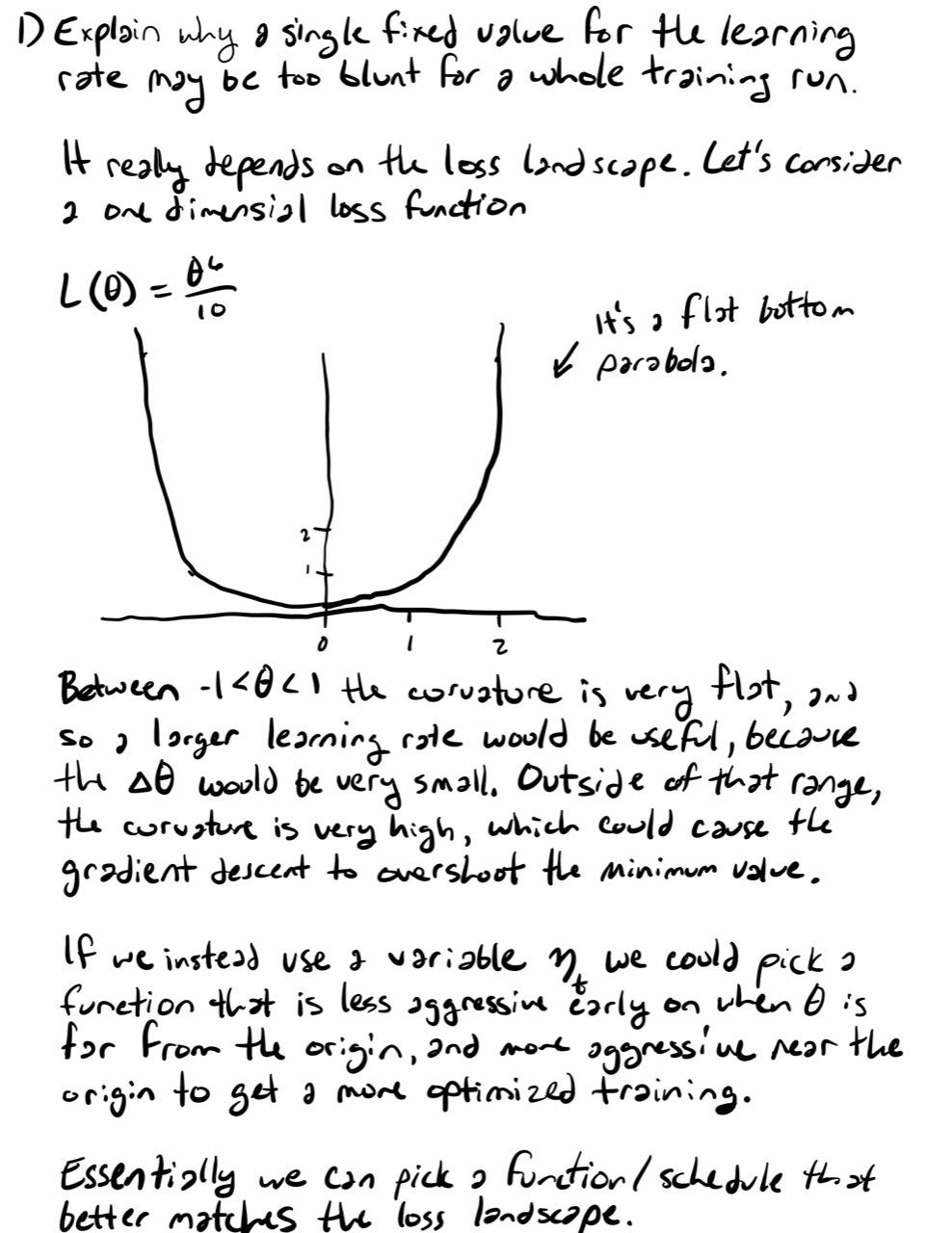
In your own words, explain why a single fixed learning rate may be too blunt for a whole training run.
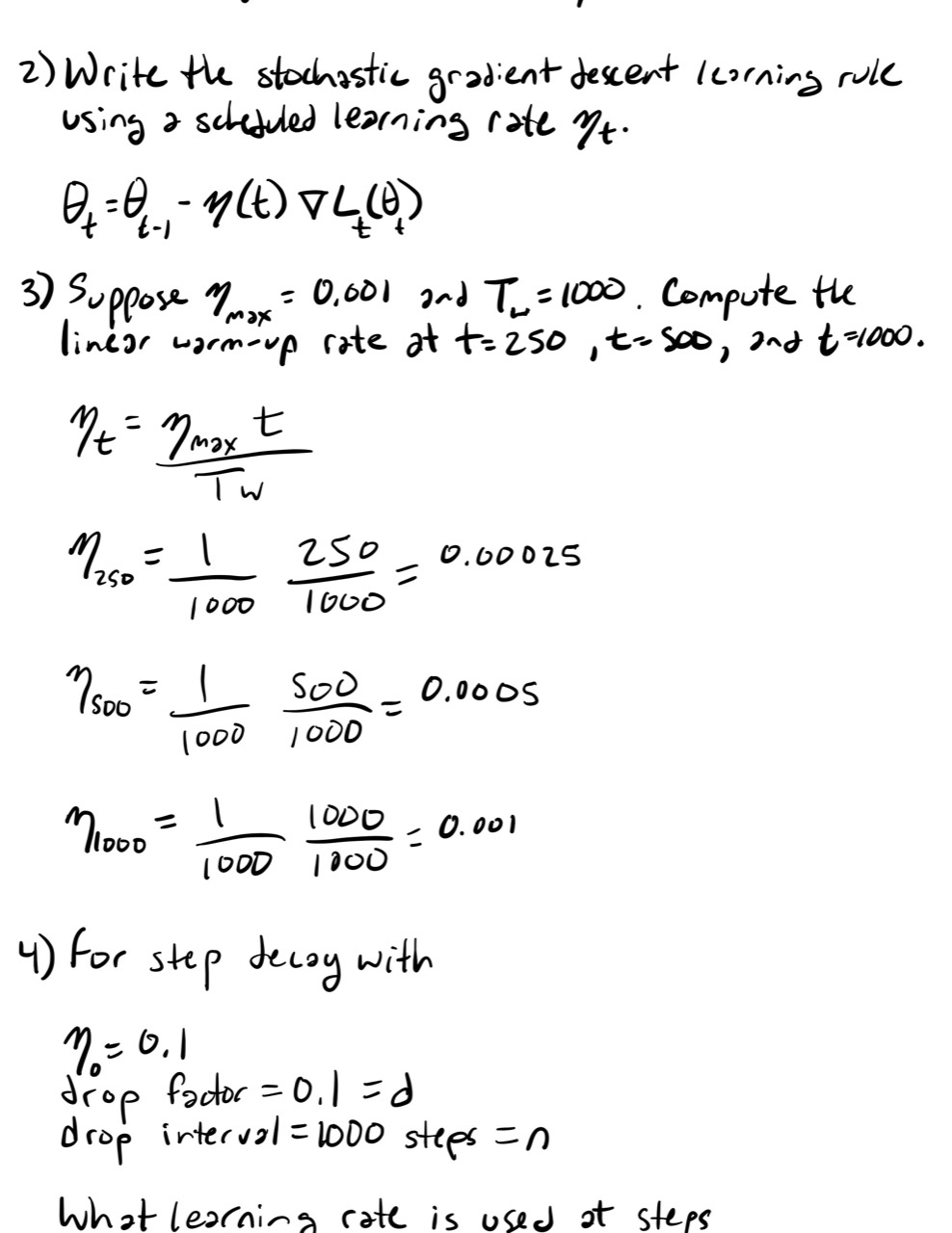
Write the SGD update rule using a scheduled learning rate $\eta_t$ .
Suppose $\eta_{max} = 0.001$ and $T_w = 1000$ . Compute the linear warmup learning rate at $t = 250$ , $t = 500$ , and $t = 1000$ .
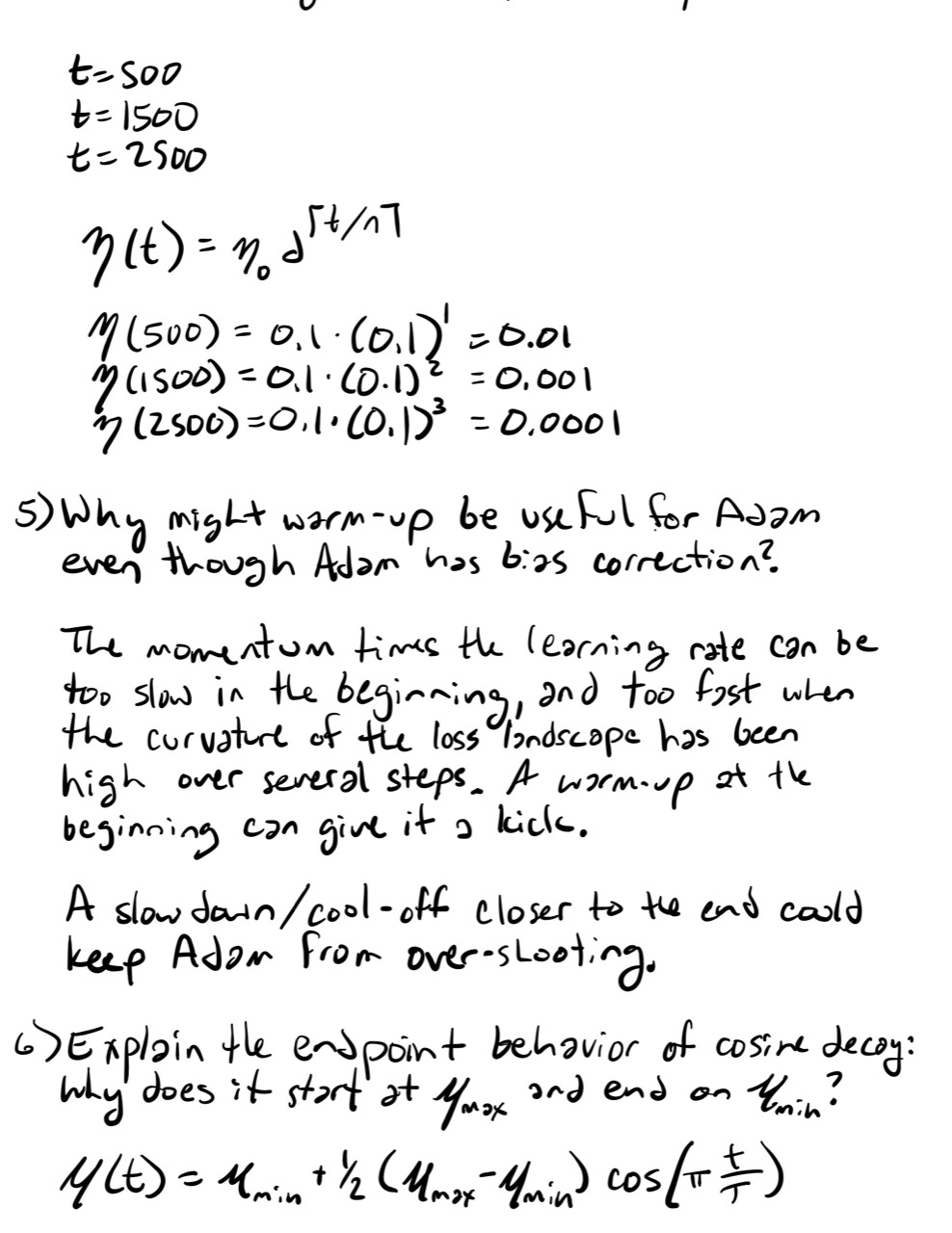
For step decay with initial learning rate $0.1$ , drop factor $0.1$ , and drop interval 1000 steps, what learning rate is used at steps 500, 1500, and 2500?
Why might warmup be useful for Adam even though Adam already has bias correction?
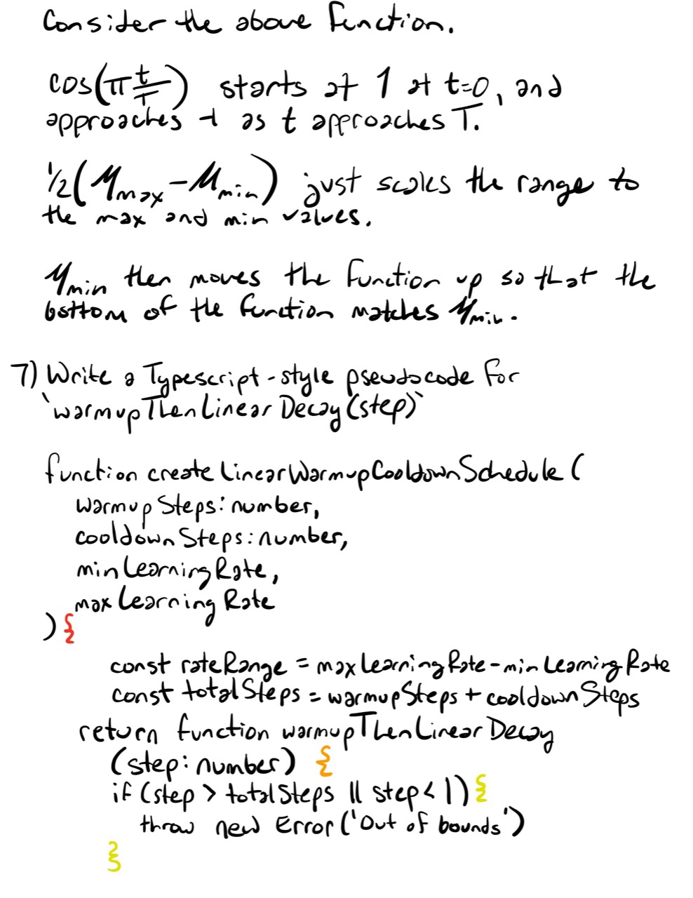
Explain the endpoint behavior of cosine decay: why does it start at $\eta_{max}$ and end at $\eta_{min}$ ?
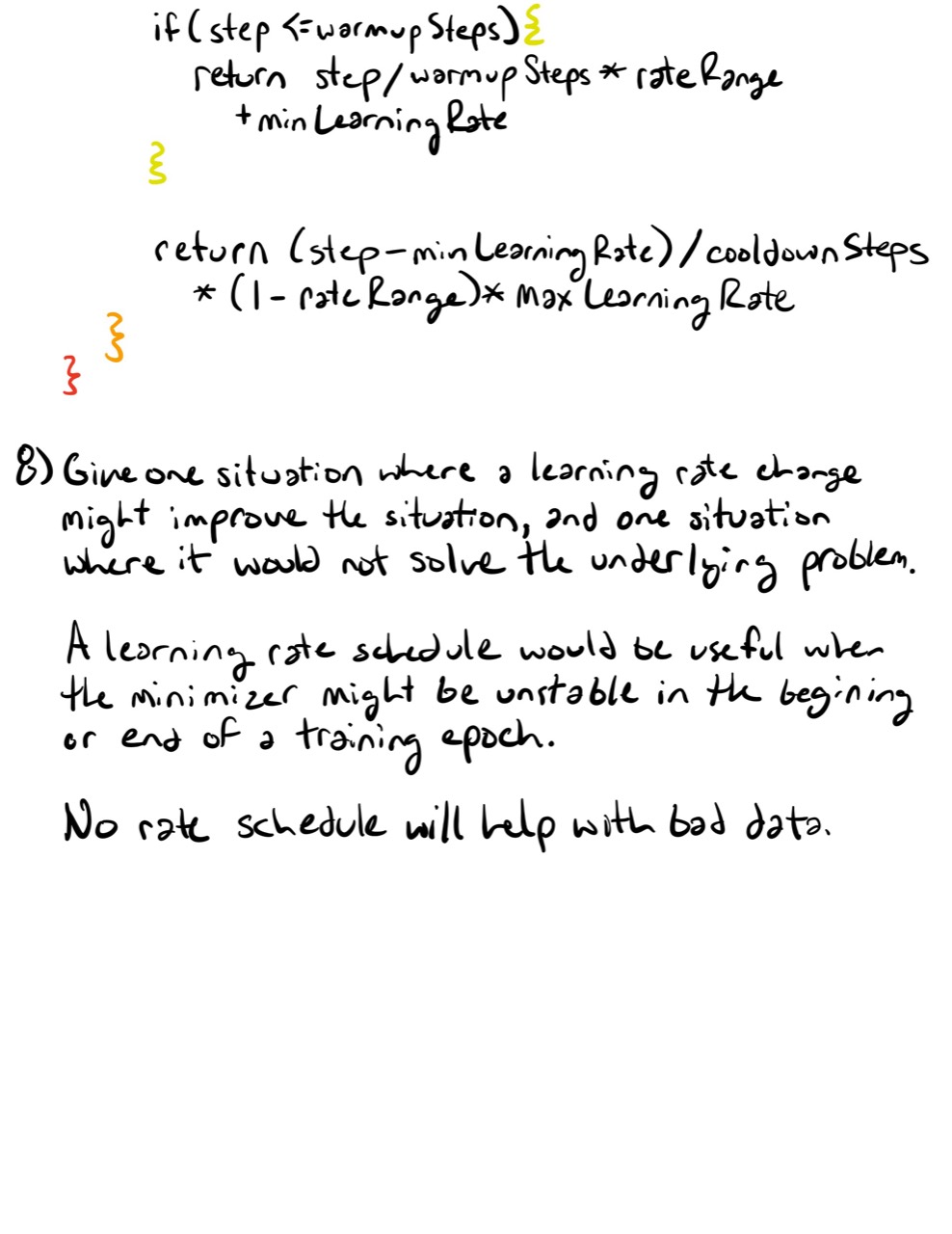
Write TypeScript-style pseudocode for a function warmupThenLinearDecay(step).
Give one situation where a learning rate schedule might improve training, and one situation where it would not solve the underlying problem.

Looking Ahead

Learning rate schedules change the step scale over time.

The next optimization question is:

What does it mean for a loss surface to be curved, and how can curvature affect optimization?

That leads to second derivatives, Hessians, and curvature.

Completed Exercises

Handwritten work submitted after completing this lesson.