Lesson 31: Hessians and Curvature

Goal

Understand curvature as the next layer of information after the gradient.

The gradient tells us:

Which direction looks downhill right here?

The Hessian tells us:

How quickly is that downhill direction changing as we move?

That matters because optimization does not only depend on direction. It also depends on the shape of the loss surface.

Motivation

Gradient descent uses first-derivative information:

\theta_{t+1} = \theta_t - \eta \nabla L(\theta_t)

The gradient points in the direction of steepest local increase, so the negative gradient points locally downhill.

But the gradient alone does not tell us whether the local surface is:

a broad shallow valley;
a narrow steep canyon;
a bowl;
a ridge;
a saddle.

Those shapes affect whether a learning rate is safe.

A step size that works in a flat direction may explode in a steep direction. A step size that is safe in a steep direction may crawl in a flat direction.

That is the optimization reason we care about curvature.

Prerequisites

Lesson 26: Gradient Descent.
Lesson 27: Stochastic Gradient Descent.
Lesson 30: Learning Rate Schedules.
Comfort with derivatives as local change.
Comfort with matrices as transformations.
Comfort with eigenvectors as special directions of a matrix.

Notation / Symbol Table

Symbol	Plain-English name	Meaning
$f(x)$	scalar function	A one-dimensional function.
$L(\theta)$	loss function	Loss as a function of model parameters.
$\theta$	parameter vector	The values the optimizer changes.
$\nabla L(\theta)$	gradient	Vector of first partial derivatives.
$f'(x)$	first derivative	Local slope in one dimension.
$f''(x)$	second derivative	How the slope is changing.
$H$	Hessian	Matrix of second partial derivatives.
$\lambda$	eigenvalue	Curvature scale in a Hessian eigenvector direction.
$v$	direction vector	A direction in parameter space.

One Dimension: Slope Versus Curvature

Start with a one-dimensional function:

f(x) = x^2

The first derivative is:

f'(x) = 2x

This tells us the slope at each point.

The second derivative is:

f''(x) = 2

This tells us that the slope changes at a constant rate.

Now compare:

g(x) = 10x^2

Then:

g'(x) = 20x

and:

g''(x) = 20

Both are bowls. But $g(x)$ is a sharper bowl than $f(x)$ .

That sharpness is curvature.

Curvature As “How Fast The Slope Changes”

A useful phrase:

The gradient tells you the current tilt. The second derivative tells you how quickly the tilt is changing.

For one-dimensional functions:

$f''(x) > 0$ means the curve bends upward like a bowl.
$f''(x) < 0$ means the curve bends downward like a hilltop.
$f''(x) = 0$ means no local quadratic bending in that direction.

This is local information. It describes the function near a point, not necessarily everywhere.

Why Curvature Affects Gradient Descent

Consider:

f(x) = ax^2

where $a > 0$ .

Then:

f'(x) = 2ax

A gradient descent update is:

x_{t+1} = x_t - \eta 2a x_t

Factor out $x_t$ :

x_{t+1} = (1 - 2a\eta)x_t

The multiplier $(1 - 2a\eta)$ controls the behavior.

If $\eta$ is too large relative to $a$ , the update overshoots. If it is much too large, it diverges.

Since:

f''(x) = 2a

larger curvature means a smaller safe learning rate.

This is the link back to learning-rate schedules: the schedule changes the step size, but curvature helps explain why some step sizes are safe and others are not.

Two Dimensions: The Hessian

For a multivariable loss:

L(\theta_1, \theta_2)

there is not just one second derivative. There are second partial derivatives.

The Hessian collects them into a matrix:

H = \begin{bmatrix} \frac{\partial^2 L}{\partial \theta_1^2} & \frac{\partial^2 L}{\partial \theta_1 \partial \theta_2} \\ \frac{\partial^2 L}{\partial \theta_2 \partial \theta_1} & \frac{\partial^2 L}{\partial \theta_2^2} \end{bmatrix}

Read the diagonal entries as same-coordinate curvature:

how the slope changes as $\theta_1$ changes;
how the slope changes as $\theta_2$ changes.

Read the off-diagonal entries as interaction curvature:

how the $\theta_1$ slope changes when $\theta_2$ changes;
how the $\theta_2$ slope changes when $\theta_1$ changes.

For smooth losses, the two mixed partials are usually equal:

\frac{\partial^2 L}{\partial \theta_1 \partial \theta_2} = \frac{\partial^2 L}{\partial \theta_2 \partial \theta_1}

So the Hessian is often symmetric.

Worked Example: Diagonal Hessian

Let:

L(x, y) = x^2 + 10y^2

The gradient is:

\nabla L(x, y) = \begin{bmatrix} 2x \\ 20y \end{bmatrix}

The Hessian is:

H = \begin{bmatrix} 2 & 0 \\ 0 & 20 \end{bmatrix}

Interpretation:

curvature in the $x$ direction is $2$ ;
curvature in the $y$ direction is $20$ ;
there is no interaction term between $x$ and $y$ .

So the surface is much steeper in the $y$ direction than in the $x$ direction.

A learning rate that is comfortable along $x$ may bounce along $y$ .

Hessian Eigenvectors: Principal Curvature Directions

Because the Hessian is a matrix, it transforms direction vectors.

When $H$ is symmetric, its eigenvectors give special directions of curvature.

If:

Hv = \lambda v

then moving in direction $v$ has curvature strength $\lambda$ .

For a Hessian:

large positive $\lambda$ means steep upward bowl direction;
small positive $\lambda$ means flat upward bowl direction;
negative $\lambda$ means downward-bending direction;
mixed positive and negative eigenvalues indicate a saddle.

This connects back to earlier linear algebra:

The Hessian is locally telling us the shape of the loss surface by decomposing it into special curvature directions.

That is the same pattern as PCA and covariance geometry: use eigenvectors to find the important directions of a quadratic-like object.

Bowls, Hills, and Saddles

At a point where the gradient is zero, curvature helps classify the point.

Gradient	Hessian behavior	Local shape
$\nabla L = 0$	all eigenvalues positive	local minimum candidate
$\nabla L = 0$	all eigenvalues negative	local maximum candidate
$\nabla L = 0$	mixed signs	saddle point
$\nabla L \ne 0$	any Hessian	not stationary; still has slope

A saddle point is especially important in high-dimensional optimization.

In one direction, it may curve upward. In another direction, it may curve downward.

So a point can have zero gradient without being a minimum.

The Local Quadratic Approximation

Near a point $\theta$ , a smooth loss can be approximated by:

L(\theta + \Delta) \approx L(\theta) + \nabla L(\theta)^T \Delta + \frac{1}{2}\Delta^T H \Delta

Symbol table for this expression:

Symbol	Meaning
$\Delta$	Small proposed movement in parameter space.
$\nabla L(\theta)^T \Delta$	First-order change predicted by the gradient.
$\frac{1}{2}\Delta^T H \Delta$	Second-order correction from curvature.

This formula says:

start with the current loss;
add what the gradient predicts;
correct that prediction using curvature.

This is why second derivatives show up in optimization theory. They describe the local quadratic bowl that the optimizer is moving through.

Why We Do Not Usually Build The Full Hessian

For a model with $n$ parameters, the Hessian is an $n \times n$ matrix.

If a model has one million parameters, the Hessian would have one trillion entries.

That is too large to store or invert directly in ordinary neural network training.

So modern optimizers usually do not build the full Hessian.

Instead, they use cheaper approximations or indirect signals:

Adam uses running squared-gradient scale.
Learning-rate schedules control the global step size over time.
Second-order methods use curvature more directly, but at higher computational cost.
Hessian-vector products can sometimes probe curvature without materializing the whole matrix.

For now, the goal is not to implement a full second-order optimizer. The goal is to understand what curvature means and why it affects training.

Connection To Programming

A Hessian for a two-variable scalar function can be represented as a 2x2 matrix.

For:

L(x, y) = x^2 + 10y^2

we can write:

function gradient(x: number, y: number): [number, number] {
  return [2 * x, 20 * y];
}

function hessian(): [[number, number], [number, number]] {
  return [
    [2, 0],
    [0, 20],
  ];
}

To inspect curvature along a direction $v$ , compute:

v^T H v

For a unit vector $v$ , this gives the curvature in that direction.

function curvatureInDirection(
  hessian: [[number, number], [number, number]],
  direction: [number, number],
): number {
  const [x, y] = direction;
  const hx = hessian[0][0] * x + hessian[0][1] * y;
  const hy = hessian[1][0] * x + hessian[1][1] * y;

  return x * hx + y * hy;
}

For direction [1, 0], the curvature is 2.

For direction [0, 1], the curvature is 20.

What Curvature Does Not Solve

Curvature information does not choose the right model.

It does not fix bad data.

It does not make nonconvex optimization easy.

It does not remove the need for validation checks.

It does explain why some regions of the loss surface are easy to optimize and others are awkward.

Why Hessians Show Up In ML

Hessians and curvature show up because training behavior depends on the local geometry of the loss surface.

They help explain:

why learning rates can be unstable;
why valleys can be slow to traverse;
why saddle points are not minima;
why coordinatewise scaling can help;
why second-order methods are attractive but expensive;
why flatness and sharpness are discussed in generalization.

You do not need the full Hessian to train a neural network today. But you do need the concept to understand many optimizer arguments.

Summary

The gradient is first-order information:

\nabla L(\theta)

It tells us local slope.

The Hessian is second-order information:

H_{ij} = \frac{\partial^2 L}{\partial \theta_i \partial \theta_j}

It tells us local curvature.

The eigenvectors of the Hessian identify special curvature directions:

Hv = \lambda v

The eigenvalues tell us how curved the loss is in those directions.

Curvature matters because the same learning rate can be safe in flat directions and unstable in steep directions.

Exercises

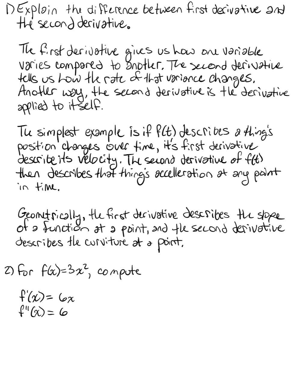
In your own words, explain the difference between a first derivative and a second derivative.
For $f(x) = 3x^2$ , compute $f'(x)$ and $f''(x)$ .
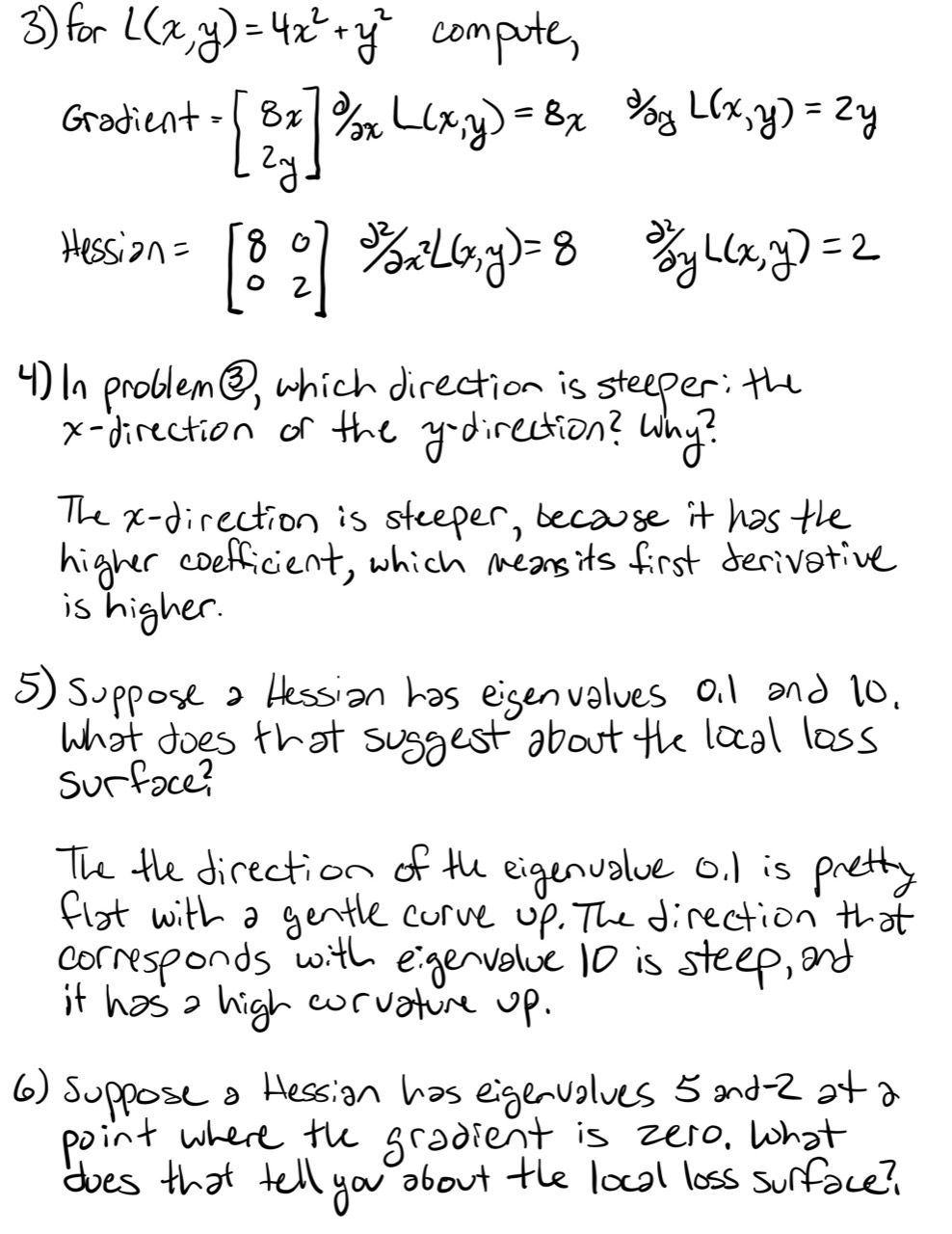
For $L(x, y) = 4x^2 + y^2$ , compute the gradient and Hessian.
In Problem 3, which direction is steeper: the $x$ direction or the $y$ direction? Why?
Suppose a Hessian has eigenvalues $10$ and $0.1$ . What does that suggest about the local loss surface?
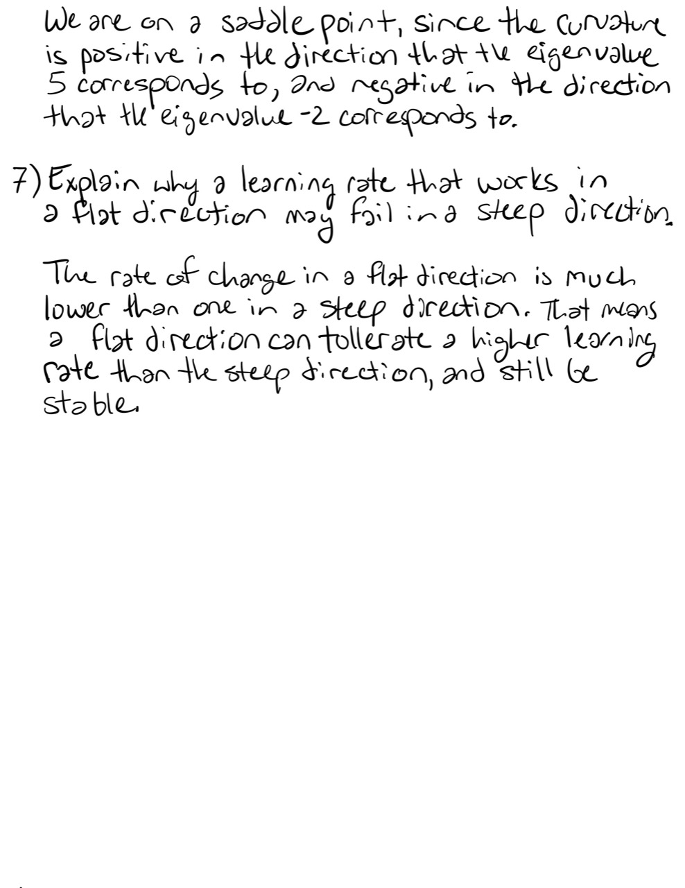
Suppose a Hessian has eigenvalues $5$ and $-2$ at a point where the gradient is zero. What kind of point is this likely to be?
Explain why a learning rate that works in a flat direction might fail in a steep direction.
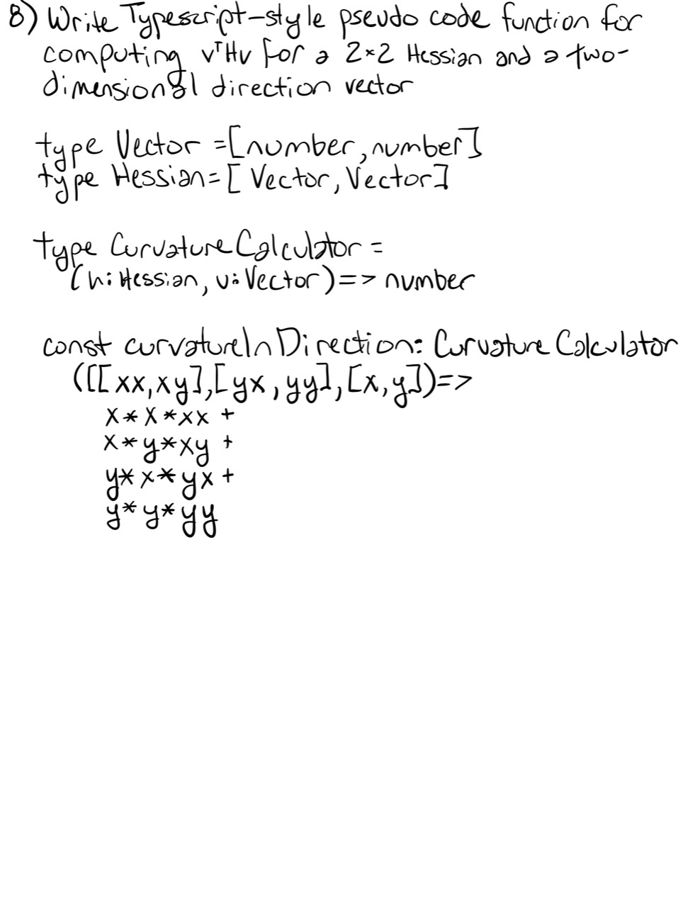
Write TypeScript-style pseudocode for computing $v^T H v$ for a 2x2 Hessian and a 2D direction vector.

Looking Ahead

Curvature lets us distinguish broad bowls, steep valleys, and saddle points.

The next optimization question is:

When can we guarantee that local downhill movement behaves nicely?

That leads to convexity.

Completed Exercises

Handwritten work submitted after completing this lesson.