Goal
Understand the geometric property that turns local downhill information into a global guarantee.
Convexity is the reason some optimization problems are unusually well behaved:
In a convex problem, a local minimum cannot secretly be worse than another distant minimum.
That does not mean optimization is always fast or numerically easy. It means the landscape has no deceptive local valleys.
Motivation
Gradient descent only sees local information.
At the current point, it asks:
For an arbitrary nonconvex function, following local downhill directions can lead to:
- a poor local minimum;
- a saddle point;
- a flat plateau;
- a complicated region with many valleys.
Convexity removes one major source of ambiguity.
For a convex function:
- every local minimum is global;
- every stationary point is a global minimum;
- chords lie above the graph;
- curvature is never negative.
These statements are different views of the same underlying shape.
Notation / Symbol Table
| Symbol | Plain-English name | Meaning |
|---|---|---|
| set | A collection of allowed points. | |
| function | A scalar-valued objective or loss. | |
| points | Two points in the domain. | |
| interpolation weight | A number satisfying . | |
| convex combination | A point on the line segment joining and . | |
| gradient | Local first-order change at . | |
| Hessian | Local second-order curvature at . |
First Idea: A Convex Set Contains Its Chords
A set is convex when the straight line segment between any two points in the set remains entirely inside the set.
Formally, for every and every :
The expression
interpolates between and :
- gives ;
- gives ;
- gives the midpoint;
- intermediate values trace the segment.
Examples of convex sets
- A line.
- A filled circle or sphere.
- A rectangle.
- A half-plane.
- All of .
Examples of nonconvex sets
- A ring with a hole.
- A crescent.
- Two disconnected islands.
- The boundary of a circle without its interior.
The distinction matters in constrained optimization. Even a convex objective can become difficult if the allowed region is nonconvex.
Convex Combinations
The expression
is called a convex combination of and .
The weights are:
They have two properties:
and:
This is a weighted average.
In programming terms, it is linear interpolation:
function lerp(a: number, b: number, t: number): number {
  return t * a + (1 - t) * b;
}
For vectors, the same operation is applied componentwise.
Convex Functions: The Graph Lies Below Its Chords
A function is convex when, for every pair of points and and every :
This is the convexity inequality, also called the chord inequality.
Read the two sides as:
- left side: evaluate the function at an interpolated input;
- right side: interpolate between the two endpoint function values.
For a convex function, the graph lies at or below the straight chord joining any two graph points.
Programming analogy
There are two possible orders:
interpolate inputs, then evaluateversus:
evaluate endpoints, then interpolate outputsConvexity says:
f(interpolate inputs) <= interpolate f(outputs)This inequality is the formal version of “bowl-shaped.”
Worked Example:
Choose:
The interpolated input is:
Evaluate the left side:
Evaluate and interpolate the endpoint values:
Therefore:
The midpoint of the curve lies below the midpoint of the chord.
One numerical example does not prove global convexity, but it illustrates the definition.
A Nonconvex Example
Consider:
Using the same points:
while:
Convexity would require:
which is false.
The graph lies above its chord, so is concave rather than convex.
Convex Versus Strictly Convex
A function is strictly convex when the chord inequality is strict for distinct points and interior weights:
for and .
Why the distinction matters:
- A convex function may have a flat interval of global minima.
- A strictly convex function has at most one global minimizer.
Example:
is strictly convex.
A constant function is convex but not strictly convex.
First-Derivative View: Tangent Lines Stay Below
For a differentiable convex function:
In one dimension:
The right side is the tangent-line approximation at .
Convexity says the tangent line never rises above the function.
This gives another geometric picture:
Every local linear approximation underestimates a convex function globally.
That is stronger than merely being bowl-shaped near one point.
Why A Stationary Point Is Global
Suppose is a stationary point:
Apply the first-order convexity condition:
Since the gradient is zero:
for every .
Therefore is a global minimum.
This is the central optimization guarantee.
No search over distant regions is needed to rule out a lower valley: convexity already rules one out.
Second-Derivative View: Nonnegative Curvature
For a twice-differentiable one-dimensional function, convexity is equivalent to:
throughout the domain.
Examples:
has:
so it is strictly convex.
has:
so it is convex, even though the second derivative is zero at .
This shows an important subtlety:
Strict convexity does not require at every point.
Multivariable View: Positive Semidefinite Hessian
For a twice-differentiable function , convexity is characterized by a positive semidefinite Hessian:
for every point and every direction vector .
Equivalently, every eigenvalue of the Hessian is nonnegative:
Interpretation:
- no direction bends downward;
- some directions may be flat;
- every local cross-section is bowl-shaped or flat.
For strict local curvature, a positive definite Hessian has:
for every nonzero .
Then all Hessian eigenvalues are positive.
Worked Example: A Convex Quadratic
Consider:
Its Hessian is:
The eigenvalues are and , both positive.
Therefore the function is strictly convex.
The minimum occurs where the gradient is zero:
which gives:
Because the function is convex, this stationary point is not merely a local candidate. It is the unique global minimum.
Worked Example With A Mixed Term
Consider:
The Hessian is:
For a symmetric matrix, positive definiteness can be checked using the leading principal minors:
and:
Here:
and:
So the Hessian is positive definite, and the function is strictly convex.
The mixed term rotates the principal curvature directions, but it does not destroy convexity.
Convexity Is Global, Curvature Is Local
The Hessian at one point tells us local curvature.
Convexity is a statement about the entire domain.
A function can have a positive semidefinite Hessian at one point and still fail to be convex elsewhere.
To establish convexity through the Hessian, the Hessian condition must hold throughout the relevant domain.
This distinction mirrors a recurring pattern:
- derivative information is local;
- optimization guarantees often require global assumptions.
Common Convex Losses
Several familiar objectives are convex in their direct prediction or parameter variables under appropriate model choices:
- Mean squared error for linear regression.
- Binary cross-entropy for logistic regression as a function of linear-model parameters.
- L1 and L2 regularization penalties.
- Hinge loss used in support vector machines.
But composition matters.
A convex loss applied to the output of a neural network does not make the training objective convex in the network parameters.
The network’s nonlinear parameterization usually creates a nonconvex objective.
What Convexity Guarantees
For a convex objective over a convex feasible set:
- every local minimum is global;
- every stationary point is globally minimizing;
- first-order conditions can certify optimality;
- averaging points remains inside the feasible region;
- many optimization algorithms have convergence guarantees.
For a strictly convex objective:
- the global minimizer is unique, when one exists.
What Convexity Does Not Guarantee
Convexity does not guarantee:
- that a minimum exists;
- that the minimum is unique unless stronger conditions hold;
- that optimization is fast;
- that the problem is well conditioned;
- that numerical errors are harmless;
- that the model generalizes well;
- that the chosen objective represents the real goal.
For example, a very narrow convex valley can still make gradient descent painfully slow.
Convexity removes deceptive local minima, not bad conditioning.
Connection To Gradient Descent
For a smooth convex function, gradient descent is not wandering among unrelated valleys.
Each step uses local information, but the global geometry makes that information trustworthy.
The update remains:
Convexity tells us what the landscape permits.
Smoothness and curvature bounds tell us which learning rates are safe and how quickly convergence can occur.
These assumptions play different roles:
| Property | What it controls |
|---|---|
| Convexity | No bad local minima. |
| Strict convexity | At most one minimizer. |
| Smoothness | Gradient does not change too abruptly. |
| Strong convexity | Bowl has a minimum curvature floor. |
| Condition number | Difficulty caused by unequal curvature directions. |
We will build these distinctions gradually rather than treating “convex” as synonymous with “easy.”
Connection To Programming
A numerical chord test can look like this:
type ScalarFunction = (x: number) => number;

function convexityGap(
  f: ScalarFunction,
  x: number,
  y: number,
  t: number,
): number {
  if (t < 0 || t > 1) {
    throw new RangeError("t must lie in [0, 1]");
  }

  const interpolatedInput = t * x + (1 - t) * y;
  const interpolatedOutput = t * f(x) + (1 - t) * f(y);

  return interpolatedOutput - f(interpolatedInput);
}
For a convex function, the returned gap should be nonnegative, up to floating-point error.
This is useful as an experiment, not as a proof. Testing finitely many points cannot establish an inequality over a continuous domain.
Why Convexity Shows Up In ML
Convexity gives a clean dividing line between two kinds of optimization reasoning.
For convex models such as linear and logistic regression, we can often prove:
- the optimizer is targeting a global solution;
- stationary conditions characterize the solution;
- convergence rates under stated assumptions.
For neural networks, the objective is generally nonconvex. Convex theory still matters because it provides:
- local approximations;
- baseline guarantees;
- reusable inequalities;
- intuition for regularizers and subproblems;
- a reference point for understanding what nonconvexity removes.
Summary
A convex set contains the line segment between any two of its points:
A convex function lies below every chord:
For differentiable convex functions, tangent planes lie below the graph:
For twice-differentiable functions, convexity means nonnegative curvature in every direction:
The optimization payoff is:
Every local minimum of a convex function is global.
Exercises
-
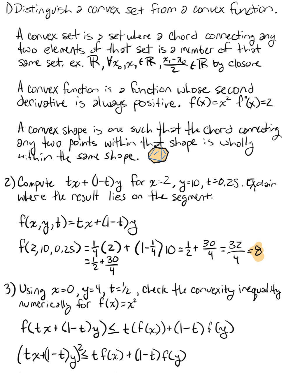
In your own words, distinguish a convex set from a convex function.
-
Compute for , , and . Explain where the result lies on the segment.
-
Using , , and , check the convexity inequality numerically for .
-
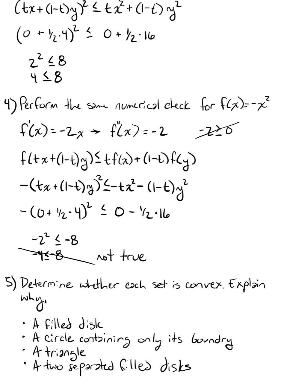
Perform the same numerical check for . Which side of the inequality fails?
-
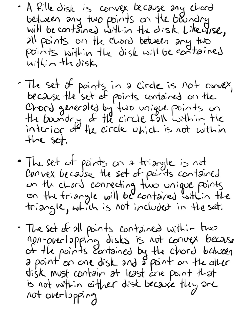
Determine whether each set is convex and explain why:
- a filled disk;
- a circle containing only its boundary;
- a rectangle;
- two separated filled disks.
-
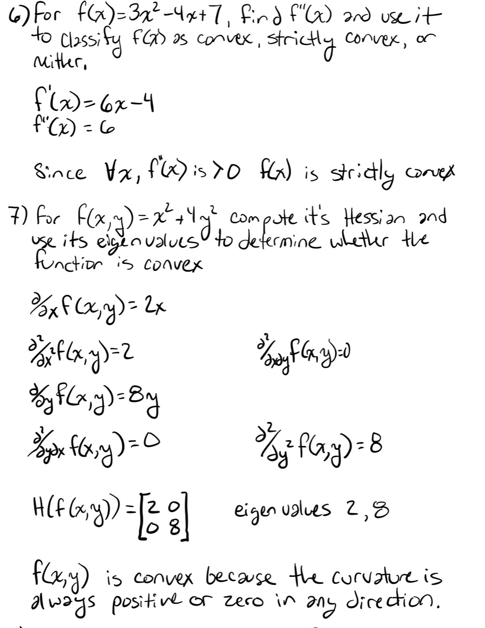
For , compute and use it to classify the function as convex, strictly convex, or neither.
-
For
compute the Hessian and use its eigenvalues to determine whether the function is convex.
-
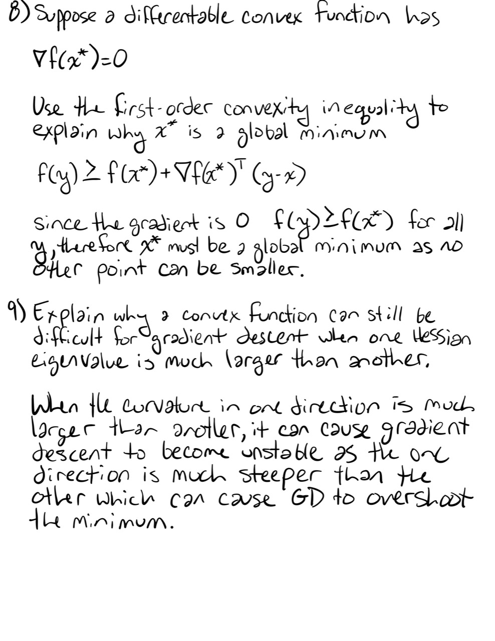
Suppose a differentiable convex function has . Use the first-order convexity inequality to explain why is a global minimum.
-
Explain why a convex function can still be difficult for gradient descent when one Hessian eigenvalue is much larger than another.
-
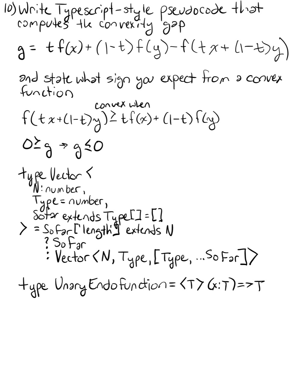
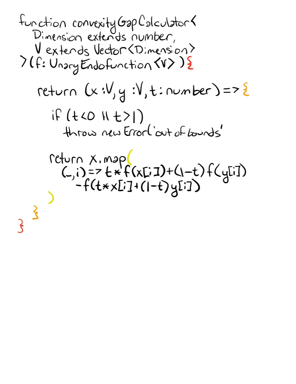
Write TypeScript-style pseudocode that computes the convexity gap
and state what sign you expect for a convex function.
Looking Ahead
Convexity tells us that the landscape has no deceptive local minima.
The next question is:
How can we optimize when parameters must satisfy explicit restrictions?
That leads to constrained optimization, feasible sets, and Lagrange multipliers.
Completed Exercises
Handwritten work submitted after completing this lesson.