Lesson 33: Constrained Optimization

Goal

Learn how to minimize an objective when not every parameter choice is allowed.

Unconstrained optimization asks:

Which point makes the objective smallest?

Constrained optimization adds a second question:

Which of those points are legal?

The answer is often found where the objective would like to move in one direction, while a constraint prevents that movement.

Motivation

Many machine-learning problems have restrictions:

probabilities must be nonnegative and sum to one;
a model may have a memory or latency budget;
portfolio weights may need to sum to a fixed total;
parameters may be bounded;
predictions may need to satisfy physical or fairness constraints.

Without constraints, gradient descent can move anywhere in parameter space. With constraints, a downhill step may leave the allowed region.

Constrained optimization separates three objects:

the objective, which says what “better” means;
the constraints, which say what is allowed;
the feasible set, which contains every allowed point.

Notation / Symbol Table

Symbol	Plain-English name	Meaning
$x$	decision variable	The point or parameter vector being chosen.
$f(x)$	objective	The scalar quantity to minimize.
$g(x)=0$	equality constraint	A rule that must hold exactly.
$h(x)\le 0$	inequality constraint	A rule that sets an allowed side of a boundary.
$C$	feasible set	All points satisfying every constraint.
$\lambda$	equality multiplier	Weight attached to an equality constraint.
$\mu$	inequality multiplier	Nonnegative weight attached to an inequality constraint.
$\mathcal{L}$	Lagrangian	Objective plus multiplier-weighted constraint terms.

The Feasible Set

Suppose we want to minimize $f(x)$ subject to constraints. The feasible set is:

C=\{x: g_i(x)=0,\ h_j(x)\le0\}

A point is feasible when it belongs to $C$ . Otherwise it is infeasible.

For example, consider:

x+y=1, \qquad x\ge0, \qquad y\ge0

The feasible set is the line segment from $(1,0)$ to $(0,1)$ . The equality restricts us to a line, and the inequalities cut that line down to a segment.

This is the same geometry as a probability vector with two entries.

Equality Versus Inequality Constraints

An equality constraint such as:

g(x)=0

usually restricts motion to a lower-dimensional surface.

An inequality constraint such as:

h(x)\le0

usually permits a region on one side of a boundary.

For example:

x^2+y^2=1

describes only the boundary of the unit circle, while:

x^2+y^2\le1

describes the filled unit disk.

The distinction matters because the set of allowed directions is different at an interior point and at a boundary point.

Why The Unconstrained Gradient Condition Is Not Enough

For an unconstrained differentiable problem, a candidate minimum often satisfies:

\nabla f(x^*)=0

But a constrained minimum may have a nonzero gradient.

Imagine minimizing height while walking along a contour drawn on a hillside. The hillside may continue downward away from the contour, but that direction is forbidden. You are finished when there is no downhill direction along the allowed path.

The constraint can balance a nonzero objective gradient.

Geometry Of A Constrained Optimum

Consider one equality constraint:

g(x)=0

At a smooth point, $\nabla g(x)$ is normal to the constraint surface. Feasible infinitesimal motion must be tangent to that surface.

At a constrained optimum, the component of $\nabla f(x)$ along every feasible tangent direction must vanish. Therefore $\nabla f(x)$ must also point in a normal direction.

With one equality constraint, the two gradients are parallel:

\nabla f(x^*)=-\lambda\nabla g(x^*)

Equivalently:

\nabla f(x^*)+\lambda\nabla g(x^*)=0

The multiplier $\lambda$ supplies the scale needed to balance the two gradients.

The Lagrangian

For the problem:

\min_x f(x) \quad \text{subject to} \quad g(x)=0

define the Lagrangian:

\mathcal{L}(x,\lambda)=f(x)+\lambda g(x)

Then solve the stationarity equations:

\nabla_x\mathcal{L}(x,\lambda)=0

and:

\frac{\partial\mathcal{L}}{\partial\lambda}=g(x)=0

The derivative with respect to $\lambda$ restores the original constraint. The derivatives with respect to $x$ express the gradient-balance condition.

The Lagrangian does not erase the constraint. It packages the objective, constraint, and balancing condition into one system of equations.

Worked Example: Closest Point On A Line

Minimize:

f(x,y)=x^2+y^2

subject to:

x+y=1

The objective is squared distance from the origin. The constraint restricts us to a line.

Write the constraint in zero form:

g(x,y)=x+y-1=0

The Lagrangian is:

\mathcal{L}(x,y,\lambda)=x^2+y^2+\lambda(x+y-1)

Differentiate:

\frac{\partial\mathcal{L}}{\partial x}=2x+\lambda=0

\frac{\partial\mathcal{L}}{\partial y}=2y+\lambda=0

\frac{\partial\mathcal{L}}{\partial\lambda}=x+y-1=0

The first two equations imply:

x=y

Substitute into the constraint:

2x=1

so:

x=y=\frac12

The constrained optimum is $(\frac12,\frac12)$ . The unconstrained minimum $(0,0)$ is lower, but it is not feasible.

What The Multiplier Means

The multiplier is more than an algebraic helper.

Suppose the constraint depends on a budget $b$ :

g(x)=b

Under suitable regularity conditions, the optimal multiplier measures how much the best objective value changes when the budget changes slightly.

This is often called a shadow price.

Intuitively:

a large multiplier means the constraint is costly or influential;
a small multiplier means relaxing the constraint changes little;
the sign depends on the chosen constraint convention.

Always interpret the sign together with the exact form used in the Lagrangian.

Inequality Constraints And Active Boundaries

Now consider:

h(x)\le0

At a candidate solution, the constraint is:

inactive if $h(x)<0$ ;
active if $h(x)=0$ .

An inactive constraint has slack: the point is safely inside the allowed region. An active constraint touches the boundary and may block further improvement.

For an inequality multiplier $\mu$ , the Karush-Kuhn-Tucker conditions include:

\mu\ge0

and complementary slackness:

\mu h(x)=0

This product says:

if $h(x)<0$ , then $\mu=0$ ;
if $\mu>0$ , then $h(x)=0$ .

Only a binding constraint exerts multiplier pressure.

KKT Conditions: The Full Checklist

For:

\min_x f(x)

subject to:

g_i(x)=0, \qquad h_j(x)\le0

define:

\mathcal{L}(x,\lambda,\mu) =f(x)+\sum_i\lambda_i g_i(x)+\sum_j\mu_j h_j(x)

The KKT conditions are:

Stationarity
$\nabla_x\mathcal{L}(x,\lambda,\mu)=0$
Primal feasibility
$g_i(x)=0, \qquad h_j(x)\le0$
Dual feasibility
$\mu_j\ge0$
Complementary slackness
$\mu_jh_j(x)=0$

These are candidate conditions in general. For convex problems under appropriate regularity assumptions, they can certify global optimality.

That connection is why Lesson 32 matters: convexity turns local-looking KKT equations into powerful global certificates.

Hard Constraints Versus Penalties

A hard-constrained problem has the form:

\min_x f(x) \quad \text{subject to} \quad g(x)=0

A penalty method instead solves something like:

\min_x f(x)+\rho\,g(x)^2

where $\rho>0$ controls how expensive violation is.

The difference is important:

a hard constraint requires exact feasibility;
a finite penalty makes violation costly but may still permit it;
increasing $\rho$ usually enforces the constraint more strongly but can worsen numerical conditioning.

Regularization often resembles a penalty, but its purpose may be to express a preference rather than approximate an inviolable rule.

Projected Gradient Descent

Another strategy is to take an ordinary gradient step and project back onto the feasible set:

z_{t+1}=x_t-\eta\nabla f(x_t)

x_{t+1}=\Pi_C(z_{t+1})

Here $\Pi_C$ means the closest feasible point in $C$ under the chosen distance.

This connects directly to earlier projection lessons:

Optimize in the ambient space, then use projection to restore feasibility.

When $C$ is convex, the Euclidean projection is uniquely defined. For complicated sets, computing the projection may itself be an optimization problem.

Connection To Probability

A categorical probability vector $p$ with $n$ entries satisfies:

p_i\ge0

and:

\sum_{i=1}^n p_i=1

These constraints define the probability simplex, a convex feasible set.

Softmax handles these constraints through parameterization: unconstrained logits are mapped automatically to positive values that sum to one.

This reveals a fourth strategy beyond Lagrangians, penalties, and projection:

Reparameterize the problem so every parameter value automatically produces a feasible solution.

Connection To Machine Learning

Constrained optimization appears when we:

normalize probability distributions;
limit a model norm or resource budget;
impose nonnegative parameters;
train with fairness or safety restrictions;
enforce conservation laws in scientific machine learning;
solve the support-vector-machine optimization problem.

Different constraints call for different tools:

Strategy	Core idea	Main tradeoff
Lagrangian	Balance objective and constraints with multipliers.	Requires solving a coupled system.
Penalty	Charge the objective for violation.	Finite penalties may remain infeasible.
Projection	Return each step to the feasible set.	Projection may be expensive.
Reparameterization	Make infeasible states impossible.	Can change geometry or be hard to design.

Connection To Programming

For a scalar equality constraint, a Lagrangian helper can keep the roles explicit:

type ScalarField = (x: readonly number[]) => number;

function lagrangian(
  objective: ScalarField,
  constraint: ScalarField,
  x: readonly number[],
  lambda: number,
): number {
  return objective(x) + lambda * constraint(x);
}

For the worked example:

const objective: ScalarField = ([x, y]) => x ** 2 + y ** 2;
const constraint: ScalarField = ([x, y]) => x + y - 1;

Notice the types:

the input is a vector;
both functions return one scalar;
the multiplier is a scalar for one scalar constraint.

Keeping those types separate prevents the coordinatewise mistake of treating a scalar-valued objective as though it returned one value per coordinate.

Common Mistakes

Forgetting zero form

Before building a Lagrangian, rewrite an equality as:

g(x)=0

Finding a stationary point but not checking feasibility

A solution to the gradient equations is irrelevant if it violates the original constraints.

Treating every inequality as active

An inequality may have slack. Complementary slackness determines whether its multiplier can be nonzero.

Assuming KKT always proves global optimality

KKT conditions need assumptions. Convexity and regularity conditions are what turn them into a global certificate.

Confusing a penalty with a hard constraint

A large penalty discourages violation. It does not automatically make violation impossible.

Summary

Constrained optimization minimizes an objective over a feasible set:

\min_{x\in C}f(x)

Equality constraints define surfaces, while inequalities define allowed sides of boundaries.

At a smooth equality-constrained optimum, the objective gradient is balanced by constraint gradients:

\nabla f(x^*)+\lambda\nabla g(x^*)=0

The Lagrangian packages this balance:

\mathcal{L}(x,\lambda)=f(x)+\lambda g(x)

For inequalities, KKT conditions add nonnegative multipliers and complementary slackness.

Convexity is the bridge from candidate conditions to global guarantees.

Exercises

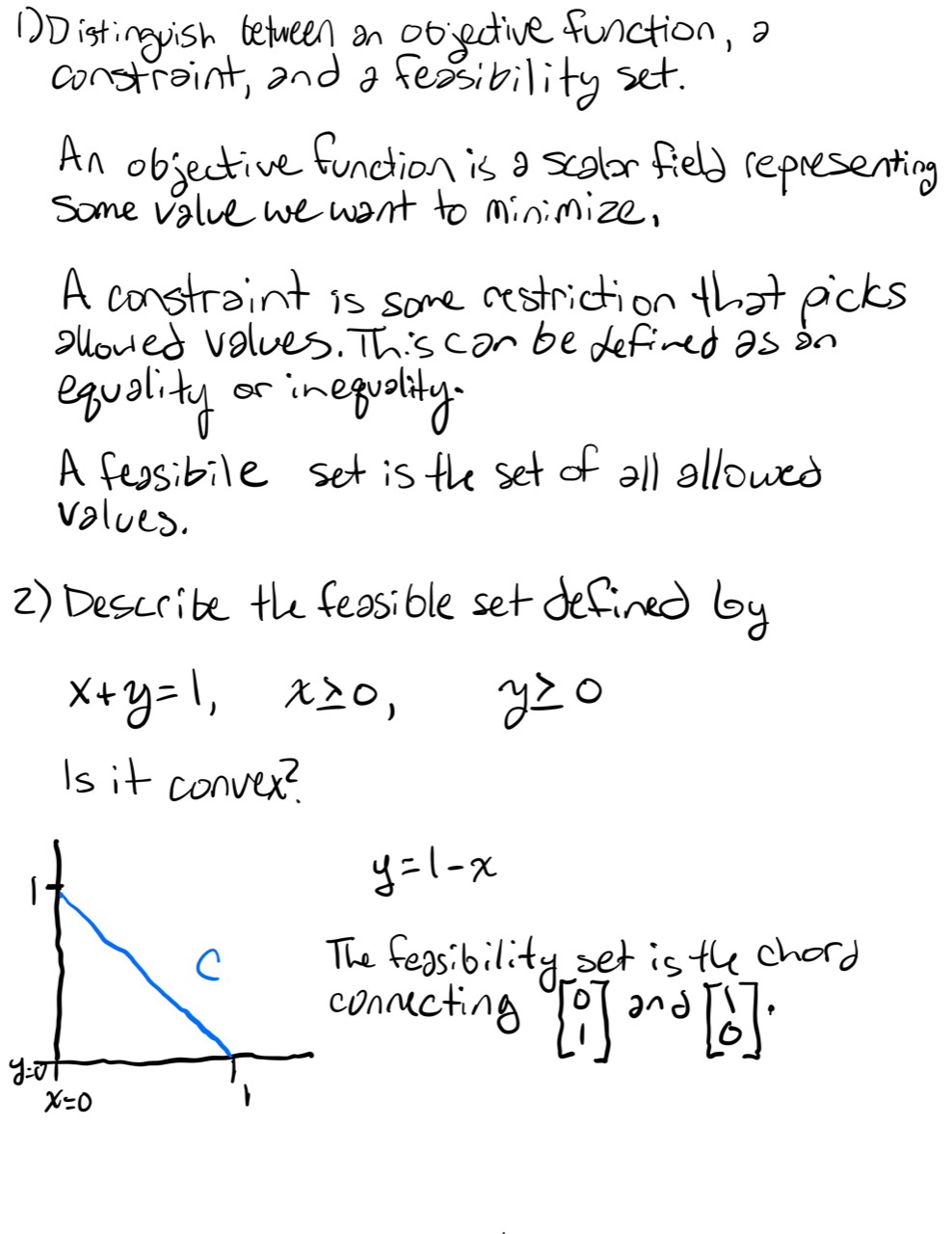
In your own words, distinguish an objective function, a constraint, and a feasible set.
Describe the feasible set defined by $x+y=1$ , $x\ge0$ , and $y\ge0$ . Is it convex?
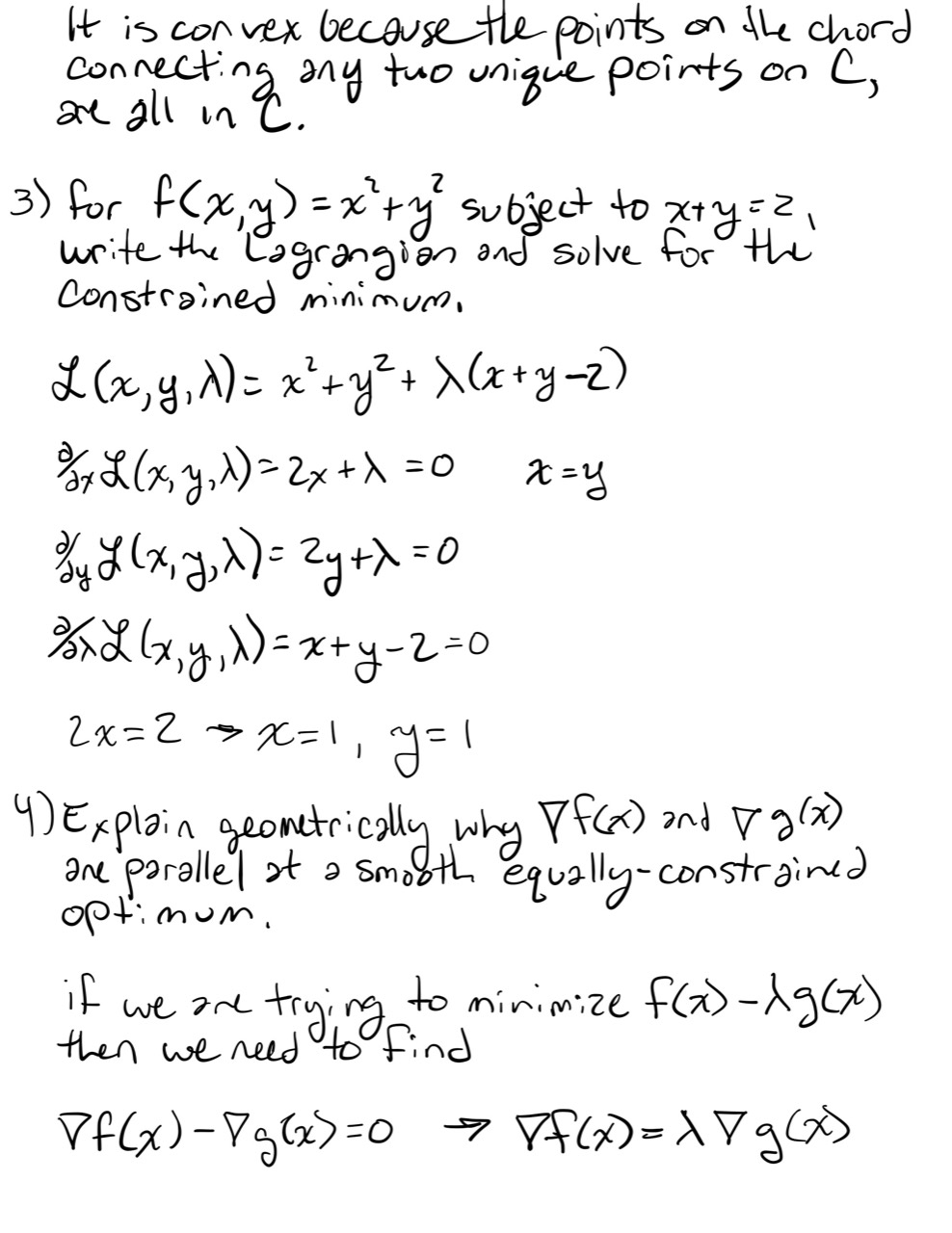
For $f(x,y)=x^2+y^2$ subject to $x+y=2$ , write the Lagrangian and solve for the constrained minimum.
Explain geometrically why $\nabla f$ and $\nabla g$ are parallel at a smooth equality-constrained optimum.
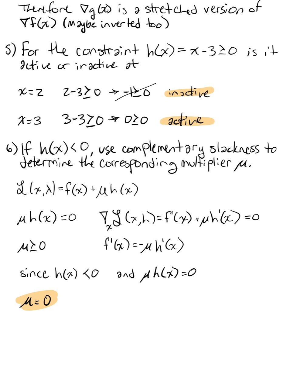
For the constraint $h(x)=x-3\le0$ , classify it as active or inactive at $x=2$ and at $x=3$ .
If $h(x)<0$ , use complementary slackness to determine the corresponding multiplier $\mu$ .
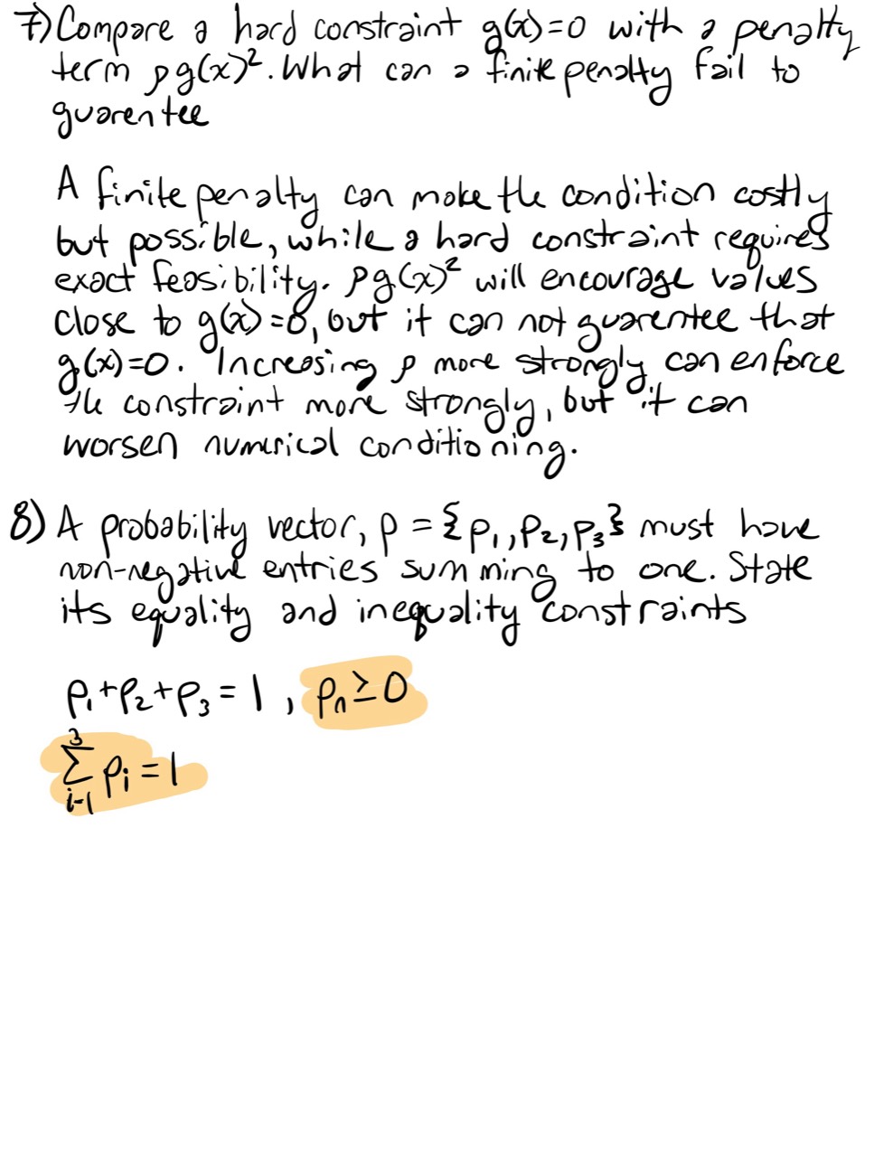
Compare a hard constraint $g(x)=0$ with the penalty term $\rho g(x)^2$ . What can a finite penalty fail to guarantee?
A probability vector $p=(p_1,p_2,p_3)$ must have nonnegative entries summing to one. State its equality and inequality constraints.
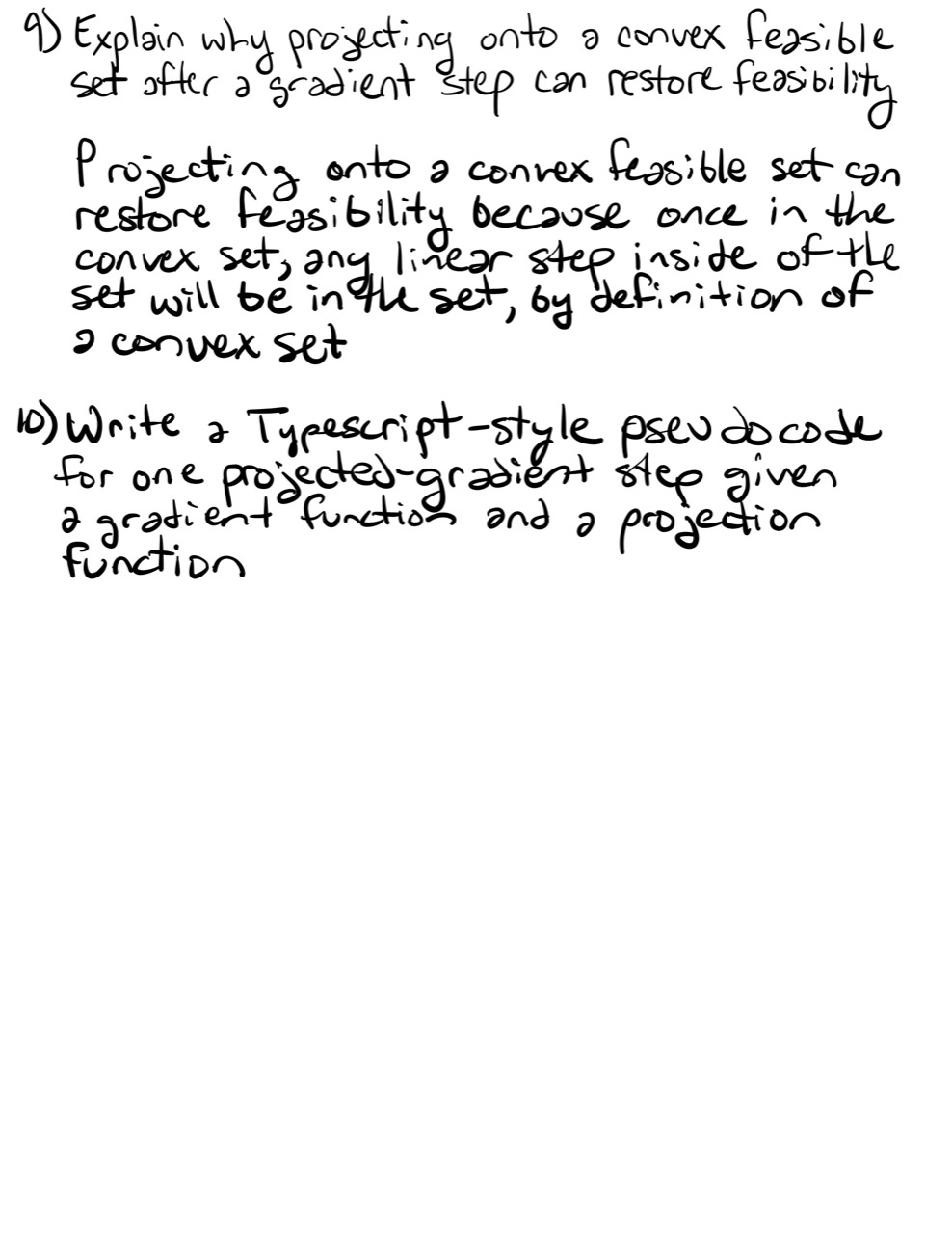
Explain why projecting onto a convex feasible set after a gradient step can restore feasibility.
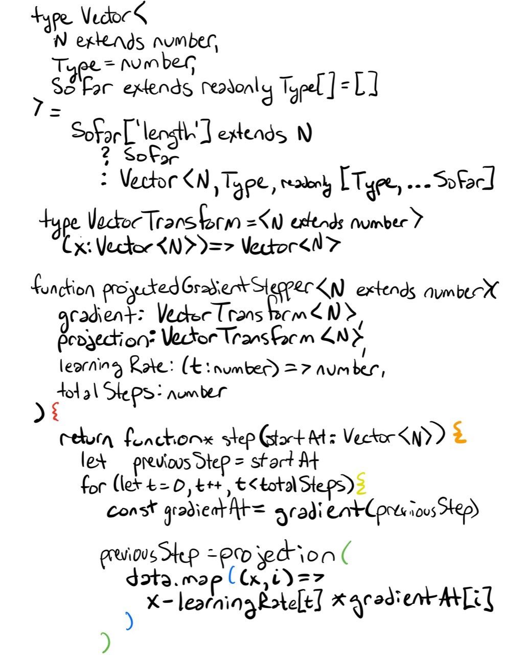
Write TypeScript-style pseudocode for one projected-gradient step given a gradient function and a projection function.

Looking Ahead

Lagrange multipliers rely on gradients of functions with several inputs.

The next lessons will slow down and formalize that machinery: partial derivatives, gradients as local linear maps, and Jacobians for vector-valued functions.

Completed Exercises

Handwritten work submitted after completing this lesson.