Lesson 34: Partial Derivatives

Goal

Learn how to ask a precise local question about a function with several inputs:

If I change only this input, how does the output respond?

That question is answered by a partial derivative.

Motivation

A machine-learning loss usually depends on many parameters:

L(\theta_1,\theta_2,\ldots,\theta_n)

Training needs to know how sensitive the loss is to each parameter. Partial derivatives isolate those coordinate-by-coordinate effects.

They are the entries from which gradients, Jacobians, and backpropagation are built.

Intuition: One Knob At A Time

Imagine a sound mixer with several knobs. The output volume depends on all of them, but you can study one knob while leaving the others untouched.

For a function $f(x,y)$ :

$\partial f/\partial x$ asks how the output changes as $x$ moves while $y$ is fixed;
$\partial f/\partial y$ asks how the output changes as $y$ moves while $x$ is fixed.

The other variable does not disappear. During that derivative, it behaves like a constant.

Notation / Symbol Table

Symbol	Plain-English name	Meaning
$f(x,y)$	scalar field	A function taking two coordinates and returning one number.
$\frac{\partial f}{\partial x}$	partial derivative with respect to $x$	Local output sensitivity when only $x$ varies.
$\partial_x f$	compact partial notation	Another way to write $\frac{\partial f}{\partial x}$ .
$(a,b)$	evaluation point	The input where a derivative is measured.
$\Delta x,\Delta y$	finite input changes	Small but non-infinitesimal coordinate changes.
$df$	total differential	First-order change assembled from all coordinate sensitivities.

The rounded symbol $\partial$ is used because the function has multiple inputs and we are differentiating with respect to only one of them.

Formal Definition

For $f:\mathbb{R}^2\to\mathbb{R}$ , the partial derivative with respect to $x$ at $(a,b)$ is:

\frac{\partial f}{\partial x}(a,b) = \lim_{h\to0}\frac{f(a+h,b)-f(a,b)}{h}

Only the first coordinate changes. The second remains exactly $b$ .

Similarly:

\frac{\partial f}{\partial y}(a,b) = \lim_{h\to0}\frac{f(a,b+h)-f(a,b)}{h}

This is ordinary one-variable differentiation applied to a coordinate slice through the surface.

Worked Example: A Quadratic Surface

Let:

f(x,y)=x^2+3xy+y^2

To differentiate with respect to $x$ , treat $y$ as a constant:

\frac{\partial f}{\partial x}=2x+3y

Why?

$x^2$ contributes $2x$ ;
$3xy$ contributes $3y$ because $y$ is constant;
$y^2$ contributes $0$ because it does not change as $x$ changes.

Now hold $x$ fixed and differentiate with respect to $y$ :

\frac{\partial f}{\partial y}=3x+2y

At $(1,2)$ :

\frac{\partial f}{\partial x}(1,2)=2+6=8

\frac{\partial f}{\partial y}(1,2)=3+4=7

Near that point, the output is slightly more sensitive to motion in the $x$ coordinate than in the $y$ coordinate.

Geometry: Slicing A Surface

The graph of $z=f(x,y)$ is a surface.

To see $\partial f/\partial x$ at $(a,b)$ :

freeze $y=b$ ;
intersect the surface with that vertical plane;
measure the slope of the resulting curve in the $x$ direction.

For $\partial f/\partial y$ , freeze $x=a$ and take the perpendicular slice.

Each partial derivative is a slope along one coordinate direction. It is not yet the whole gradient; it is one component of it.

Partial Derivatives Assemble Into The Gradient

For a scalar field $f:\mathbb{R}^n\to\mathbb{R}$ , the gradient collects all first partial derivatives:

\nabla f(x)= \begin{bmatrix} \frac{\partial f}{\partial x_1}\\ \frac{\partial f}{\partial x_2}\\ \vdots\\ \frac{\partial f}{\partial x_n} \end{bmatrix}

This shape distinction matters:

$f(x)$ is one scalar;
each $\partial f/\partial x_i$ is one scalar;
$\nabla f(x)$ is a vector containing those scalars.

The next lesson studies that assembled vector directly.

Partial Change Versus Total Change

A partial derivative isolates one coordinate. A real input change may move several coordinates at once.

For a small displacement $(\Delta x,\Delta y)$ , the first-order output change is approximately:

\Delta f \approx \frac{\partial f}{\partial x}\Delta x + \frac{\partial f}{\partial y}\Delta y

In differential notation:

df = \frac{\partial f}{\partial x}dx + \frac{\partial f}{\partial y}dy

The partial derivatives provide local sensitivity coefficients; the coordinate changes say how much of each sensitivity is activated.

Connection To Constrained Optimization

Lesson 33 used the stationarity equation:

\nabla_x\mathcal{L}(x,\lambda)=0

For $\mathcal{L}(x,y,\lambda)$ , that compact equation expands into separate partial-derivative equations:

\frac{\partial\mathcal{L}}{\partial x}=0, \qquad \frac{\partial\mathcal{L}}{\partial y}=0

The constraint is recovered from:

\frac{\partial\mathcal{L}}{\partial\lambda}=0

Partial derivatives are therefore the mechanics underneath the Lagrange-multiplier system you already solved.

Connection To Machine Learning

Suppose a loss depends on a weight $w$ and bias $b$ :

L(w,b)

Gradient descent updates them using different partial derivatives:

w_{t+1}=w_t-\eta\frac{\partial L}{\partial w}

b_{t+1}=b_t-\eta\frac{\partial L}{\partial b}

Each derivative measures the local effect of changing one parameter while conceptually holding the others fixed. The optimizer then changes all parameters together using the assembled gradient.

Connection To Programming

A scalar field with two inputs can be represented as:

type ScalarField2 = (x: number, y: number) => number;

A centered finite-difference approximation to the $x$ partial is:

function partialX(
  f: ScalarField2,
  x: number,
  y: number,
  h = 1e-5,
): number {
  return (f(x + h, y) - f(x - h, y)) / (2 * h);
}

Notice that both function evaluations use the same $y$ . Only $x$ changes.

The corresponding $y$ partial keeps $x$ fixed:

function partialY(
  f: ScalarField2,
  x: number,
  y: number,
  h = 1e-5,
): number {
  return (f(x, y + h) - f(x, y - h)) / (2 * h);
}

These numerical approximations are useful for checking analytic derivatives, although training systems usually obtain derivatives through automatic differentiation.

Common Mistakes

Differentiating every variable

When computing $\partial f/\partial x$ , all other independent variables are held constant.

Dropping a constant factor that contains another variable

For $3xy$ , differentiating with respect to $x$ gives $3y$ , not $3$ and not $0$ .

Confusing the function with its gradient

A scalar objective returns one number. Its partial derivatives are scalar components; the gradient collects them into a vector.

Treating a partial derivative as the whole change

$\partial f/\partial x$ describes sensitivity along one coordinate direction. If several inputs move, their first-order contributions must be combined.

Ignoring the evaluation point

$\partial f/\partial x$ is generally a function. A numerical slope appears only after evaluating it at a particular input.

Exercises

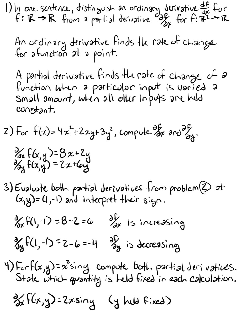
In one sentence, distinguish an ordinary derivative $df/dx$ for $f:\mathbb{R}\to\mathbb{R}$ from a partial derivative $\partial f/\partial x$ for $f:\mathbb{R}^2\to\mathbb{R}$ .
For $f(x,y)=4x^2+2xy+3y^2$ , compute $\partial f/\partial x$ and $\partial f/\partial y$ .
Evaluate both partial derivatives from Problem 2 at $(x,y)=(1,-1)$ and interpret their signs.
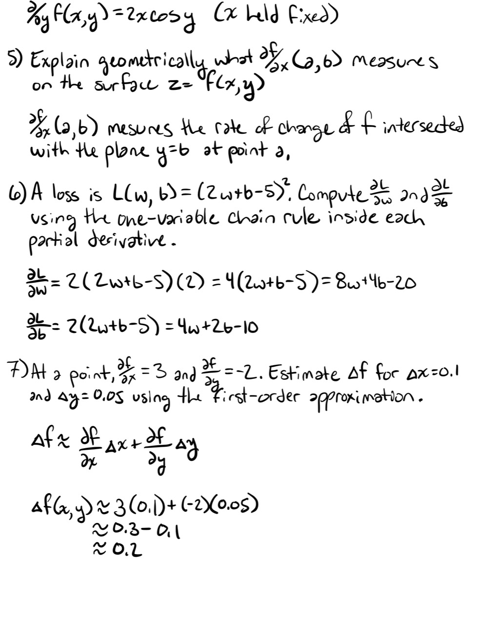
For $f(x,y)=x^2\sin y$ , compute both first partial derivatives. State explicitly which quantity is held fixed in each calculation.
Explain geometrically what $\partial f/\partial x(a,b)$ measures on the surface $z=f(x,y)$ .
A loss is $L(w,b)=(2w+b-5)^2$ . Compute $\partial L/\partial w$ and $\partial L/\partial b$ using the one-variable chain rule inside each partial derivative.
At a point, $\partial f/\partial x=3$ and $\partial f/\partial y=-2$ . Estimate $\Delta f$ for $\Delta x=0.1$ and $\Delta y=0.05$ using the first-order approximation.
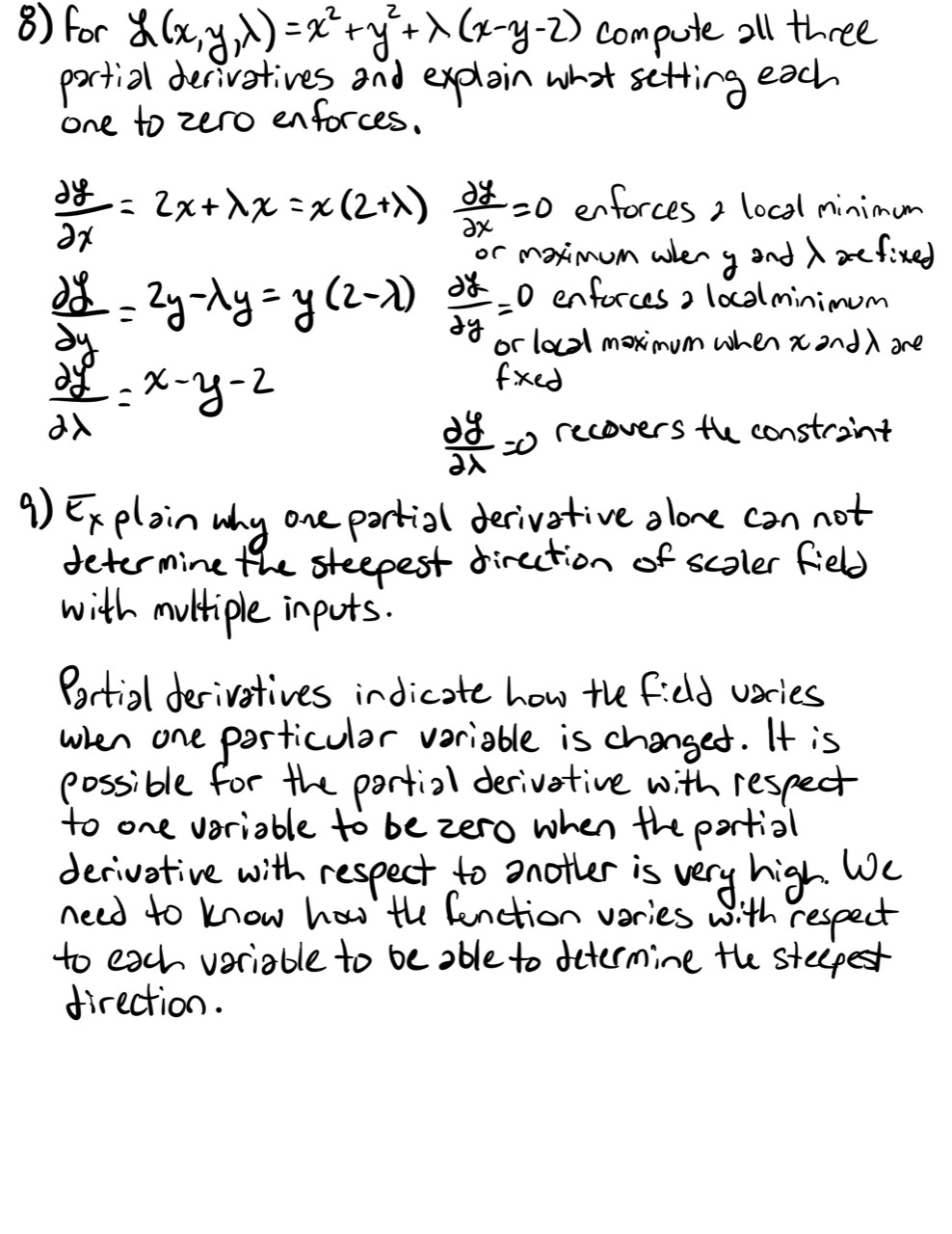
For $\mathcal{L}(x,y,\lambda)=x^2+y^2+\lambda(x+y-2)$ , compute all three partial derivatives and explain what setting each one to zero enforces.
Explain why one partial derivative alone cannot determine the steepest direction of a scalar field with multiple inputs.
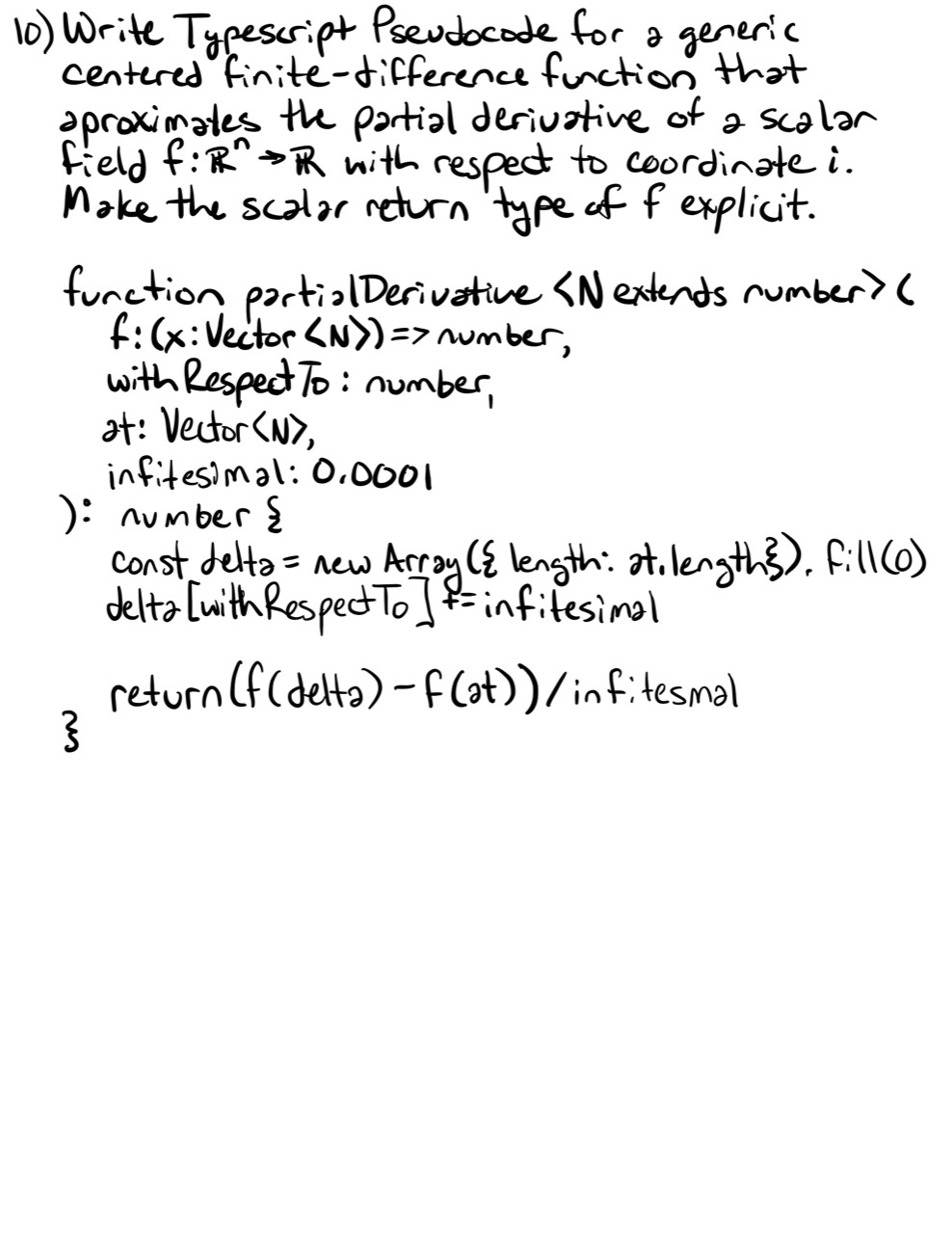
Write TypeScript-style pseudocode for a generic centered finite-difference function that approximates the partial derivative of a scalar field $f:\mathbb{R}^n\to\mathbb{R}$ with respect to coordinate $i$ . Make the scalar return type of $f$ explicit.

Summary

A partial derivative varies one input while holding the others fixed.
Geometrically, it is the slope of a coordinate slice through a surface.
Partial derivatives are scalar local sensitivities.
The gradient collects all first partial derivatives into a vector.
Small total changes combine partial sensitivities with coordinate changes.
Lagrangian stationarity and machine-learning parameter updates are built from partial derivatives.

Next Lesson

Lesson 35 assembles coordinate sensitivities into gradients and directional derivatives, then interprets the gradient as a local linear approximation.

Completed Exercises

Handwritten work submitted after completing this lesson.