Lesson 35: Gradients | Mathematics of AI

Goal

Turn many coordinate-by-coordinate sensitivities into one object that answers three questions:

How does the function change in any chosen direction?
Which unit direction increases it fastest?
What is the best linear prediction of its nearby change?

That object is the gradient.

Motivation

Lesson 34 treated a multivariable function one coordinate at a time. For a loss with thousands or billions of parameters, isolated partial derivatives are useful ingredients, but an optimizer needs them assembled.

The gradient compresses every first-order coordinate sensitivity into a vector:

\nabla L(\theta)= \begin{bmatrix} \frac{\partial L}{\partial \theta_1}\\ \vdots\\ \frac{\partial L}{\partial \theta_n} \end{bmatrix}

Once assembled, the same object predicts local change, measures slope along any direction, and supplies the update direction in gradient descent.

Intuition: A Local Sensitivity Arrow

Imagine standing on a smooth hill. The ground may rise differently in every horizontal direction.

Each partial derivative measures the slope along one coordinate axis.
The gradient combines those axis-aligned measurements into one arrow.
The arrow points toward the steepest local increase.
The arrow’s length records how steep that best ascent is.
The negative gradient points toward the steepest local decrease.

This statement compares unit directions. Without fixing direction length, any slope could be made arbitrarily large merely by scaling the direction vector.

Notation / Symbol Table

Symbol	Plain-English name	Meaning
$f:\mathbb R^n\to\mathbb R$	scalar field	A function with a vector input and scalar output.
$x$	input point	The point where local sensitivity is measured.
$\nabla f(x)$	gradient	Column vector of all coordinate partial derivatives at $x$ .
$u$	direction	A vector describing a direction of motion; usually $\lVert u\rVert=1$ .
$D_u f(x)$	directional derivative	Local rate of change along $u$ .
$\Delta x$	displacement	A small change to the input vector.
$df_x$	differential at $x$	Linear map that sends $\Delta x$ to first-order output change.
$\lVert v\rVert_2$	Euclidean norm	Length of a vector $v$ .

From Partials To A Gradient

For $f:\mathbb R^n\to\mathbb R$ , define:

\nabla f(x)= \begin{bmatrix} \frac{\partial f}{\partial x_1}(x)\\ \frac{\partial f}{\partial x_2}(x)\\ \vdots\\ \frac{\partial f}{\partial x_n}(x) \end{bmatrix}

The shape is important:

input $x$ : vector in $\mathbb R^n$ ;
output $f(x)$ : scalar in $\mathbb R$ ;
each partial derivative: scalar;
gradient $\nabla f(x)$ : vector in $\mathbb R^n$ .

The gradient has one component for every input coordinate.

Worked Example: Assemble The Components

Let:

f(x,y)=x^2+xy+2y^2

Compute the partial derivatives:

\frac{\partial f}{\partial x}=2x+y

\frac{\partial f}{\partial y}=x+4y

Assemble them:

\nabla f(x,y)= \begin{bmatrix} 2x+y\\ x+4y \end{bmatrix}

At $(1,2)$ :

\nabla f(1,2)= \begin{bmatrix} 4\\ 9 \end{bmatrix}

The function rises locally faster through the $y$ coordinate than through the $x$ coordinate, but the steepest direction is not either coordinate axis. It is the direction of the combined vector $(4,9)$ .

Directional Derivatives

A coordinate partial derivative measures change along a basis direction. A directional derivative measures change along any direction $u$ .

For a differentiable scalar field:

D_u f(x)=\nabla f(x)^T u=\nabla f(x)\cdot u

When $u$ is a unit vector, this is the slope per unit distance traveled in that direction.

For the previous example, choose the unit direction:

u=\frac{1}{\sqrt2} \begin{bmatrix} 1\\ -1 \end{bmatrix}

Then:

D_u f(1,2) = \begin{bmatrix} 4 & 9 \end{bmatrix} \frac{1}{\sqrt2} \begin{bmatrix} 1\\ -1 \end{bmatrix} =-\frac{5}{\sqrt2}

So the function decreases in that direction, even though both gradient components are positive. Directional change depends on alignment with the whole gradient.

Why The Gradient Is Steepest

For every unit vector $u$ , the Cauchy-Schwarz inequality gives:

D_u f(x) =\nabla f(x)\cdot u \le \lVert\nabla f(x)\rVert_2\lVert u\rVert_2 =\lVert\nabla f(x)\rVert_2

Equality occurs when $u$ points in the same direction as the gradient:

u=\frac{\nabla f(x)}{\lVert\nabla f(x)\rVert_2}

Therefore:

steepest unit-direction increase is along $\nabla f(x)$ ;
its rate is $\lVert\nabla f(x)\rVert_2$ ;
steepest unit-direction decrease is along $-\nabla f(x)$ ;
its rate is $-\lVert\nabla f(x)\rVert_2$ .

If $\nabla f(x)=0$ , first-order information does not prefer any direction. The point may be a minimum, maximum, saddle, or flat point; curvature or higher-order information is needed.

The Gradient As A Local Linear Approximation

For a small displacement $\Delta x$ :

f(x+\Delta x) \approx f(x)+\nabla f(x)^T\Delta x

Equivalently:

\Delta f\approx\nabla f(x)^T\Delta x

This unifies Lesson 34’s coordinate formula. In two dimensions:

\nabla f(x,y)^T \begin{bmatrix} \Delta x\\ \Delta y \end{bmatrix} = \frac{\partial f}{\partial x}\Delta x + \frac{\partial f}{\partial y}\Delta y

The dot product is not an extra trick. It is the compact form of adding every coordinate sensitivity contribution.

Gradient Vector And Differential

There is a subtle but useful distinction.

The derivative at $x$ is fundamentally the linear rule:

df_x:\Delta x\mapsto df_x(\Delta x)

For a scalar field in Euclidean coordinates:

df_x(\Delta x)=\nabla f(x)^T\Delta x

So:

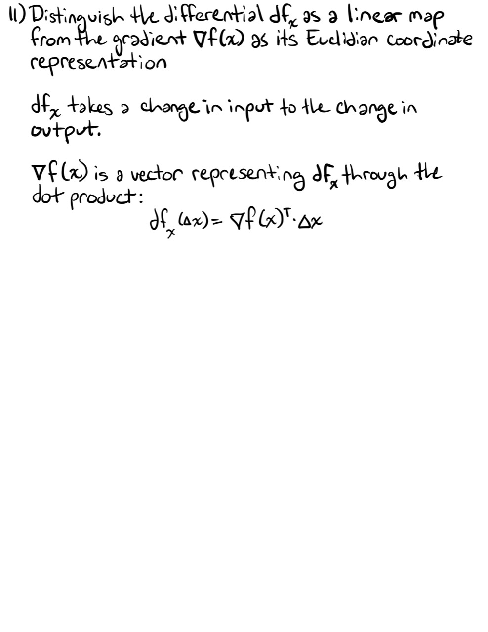
$df_x$ is a linear map from an input displacement to a scalar change;
$\nabla f(x)$ is the vector representing that map through the Euclidean dot product.

You may see the derivative called a covector because it consumes a vector and returns a scalar. In ordinary Euclidean machine-learning calculations, the inner product lets us represent that covector by the familiar gradient vector. Later matrix-calculus lessons will make the shape convention explicit.

Contours And Orthogonality

A level set keeps the function value constant:

f(x)=c

Moving tangent to a smooth level set produces no first-order change. If $t$ is a tangent direction, then:

\nabla f(x)^T t=0

Therefore the gradient is normal to the level set.

This recovers the geometry from constrained optimization: at a constrained optimum, the objective gradient cannot have a component along feasible tangent directions, so it aligns with the constraint normal.

Connection To Gradient Descent

Gradient descent applies:

\theta_{t+1}=\theta_t-\eta\nabla L(\theta_t)

The gradient supplies a local direction, while the learning rate $\eta$ chooses a step length.

Using the local linear approximation with $\Delta\theta=-\eta\nabla L(\theta)$ :

\Delta L \approx \nabla L(\theta)^T(-\eta\nabla L(\theta)) = -\eta\lVert\nabla L(\theta)\rVert_2^2

For $\eta>0$ and a nonzero gradient, the predicted first-order change is negative. This explains the sign in the update. It does not guarantee that an arbitrarily large step decreases the true loss; curvature limits how far the local approximation remains reliable.

Connection To Programming

A scalar field accepts a vector and returns one number:

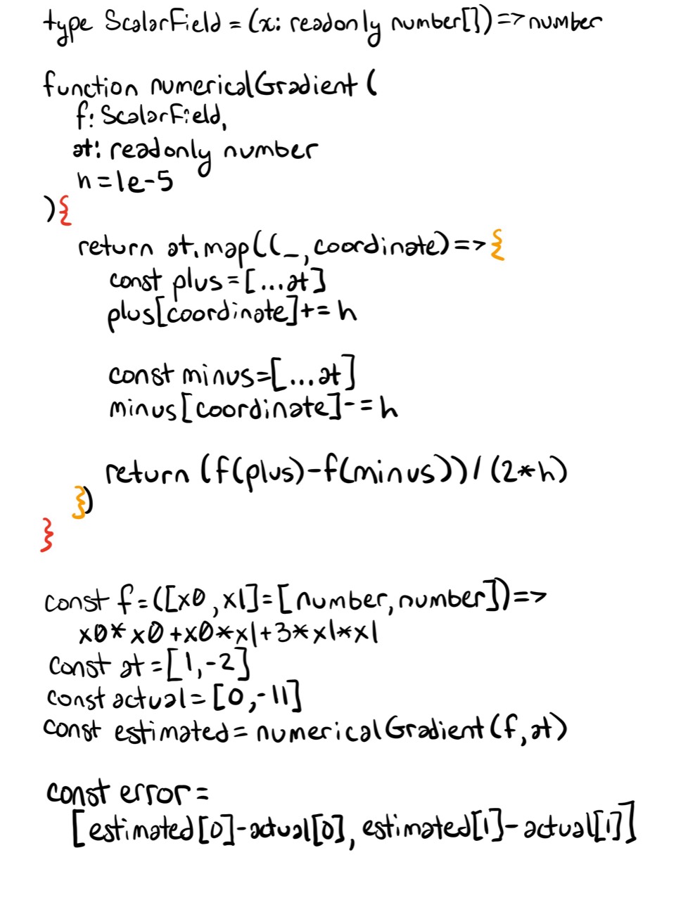
type ScalarField = (x: readonly number[]) => number;

A numerical gradient applies a centered partial-derivative check to every coordinate:

function numericalGradient(
  f: ScalarField,
  at: readonly number[],
  h = 1e-5,
): number[] {
  return at.map((_, coordinate) => {
    const plus = at.map((value, index) =>
      index === coordinate ? value + h : value,
    );
    const minus = at.map((value, index) =>
      index === coordinate ? value - h : value,
    );

    return (f(plus) - f(minus)) / (2 * h);
  });
}

Each pair of evaluations perturbs the original point at. The output array has the same length as the input because a scalar field’s gradient has one component per input coordinate.

Finite differences are useful for checking a derived or automatically computed gradient. They are approximate and require two function evaluations per coordinate, so modern training systems normally use automatic differentiation instead.

Common Mistakes

Treating the gradient as a scalar

Each partial derivative is scalar; the gradient is the vector containing all of them.

Forgetting to evaluate at a point

$\nabla f(x)$ may be a vector-valued formula. A numerical direction appears only after substituting a point.

Using a non-unit direction without tracking scale

$\nabla f(x)^T v$ scales when $v$ is scaled. Normalize the direction when asking for slope per unit distance or comparing directions.

Saying the gradient always points downhill

The gradient points toward steepest local increase. Its negative points toward steepest local decrease.

Assuming a zero gradient proves a minimum

A zero gradient identifies a stationary point. Hessian or higher-order information is needed to classify it.

Confusing a local prediction with a global guarantee

The gradient is first-order local information. Large steps can cross into a region with different slope or curvature.

Exercises

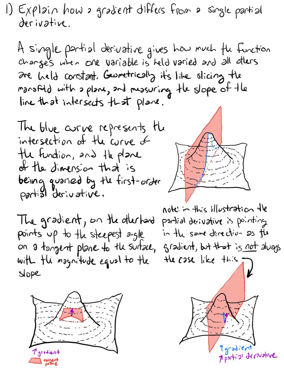
In one sentence, explain how a gradient differs from a single partial derivative.
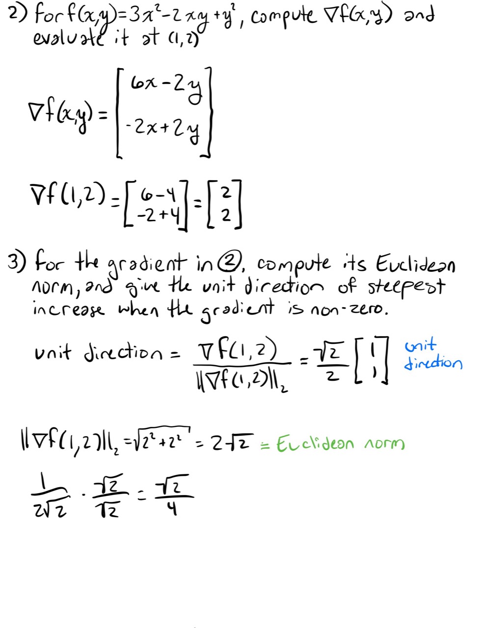
For $f(x,y)=3x^2-2xy+y^2$ , compute $\nabla f(x,y)$ and evaluate it at $(1,2)$ .
For the gradient from Problem 2, compute its Euclidean norm at $(1,2)$ and give the unit direction of steepest increase when the gradient is nonzero.
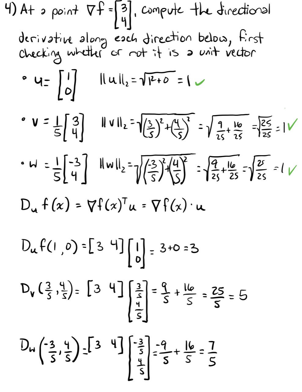
At a point, $\nabla f=[3,-4]^T$ . Compute the directional derivative along each direction below, first checking whether it is a unit vector:
- $u=[1,0]^T$
- $v=[3,4]^T/5$
- $w=[-3,4]^T/5$
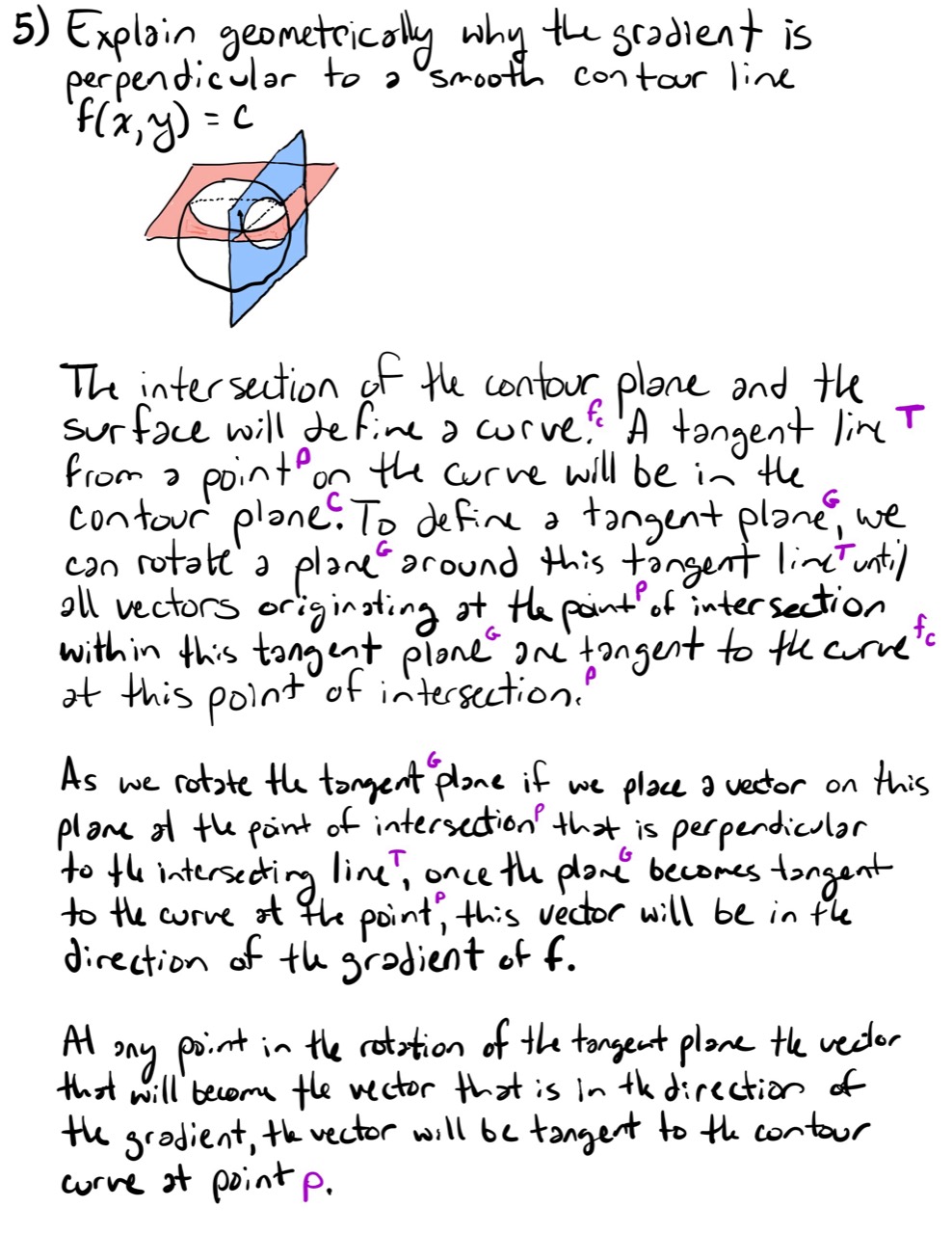
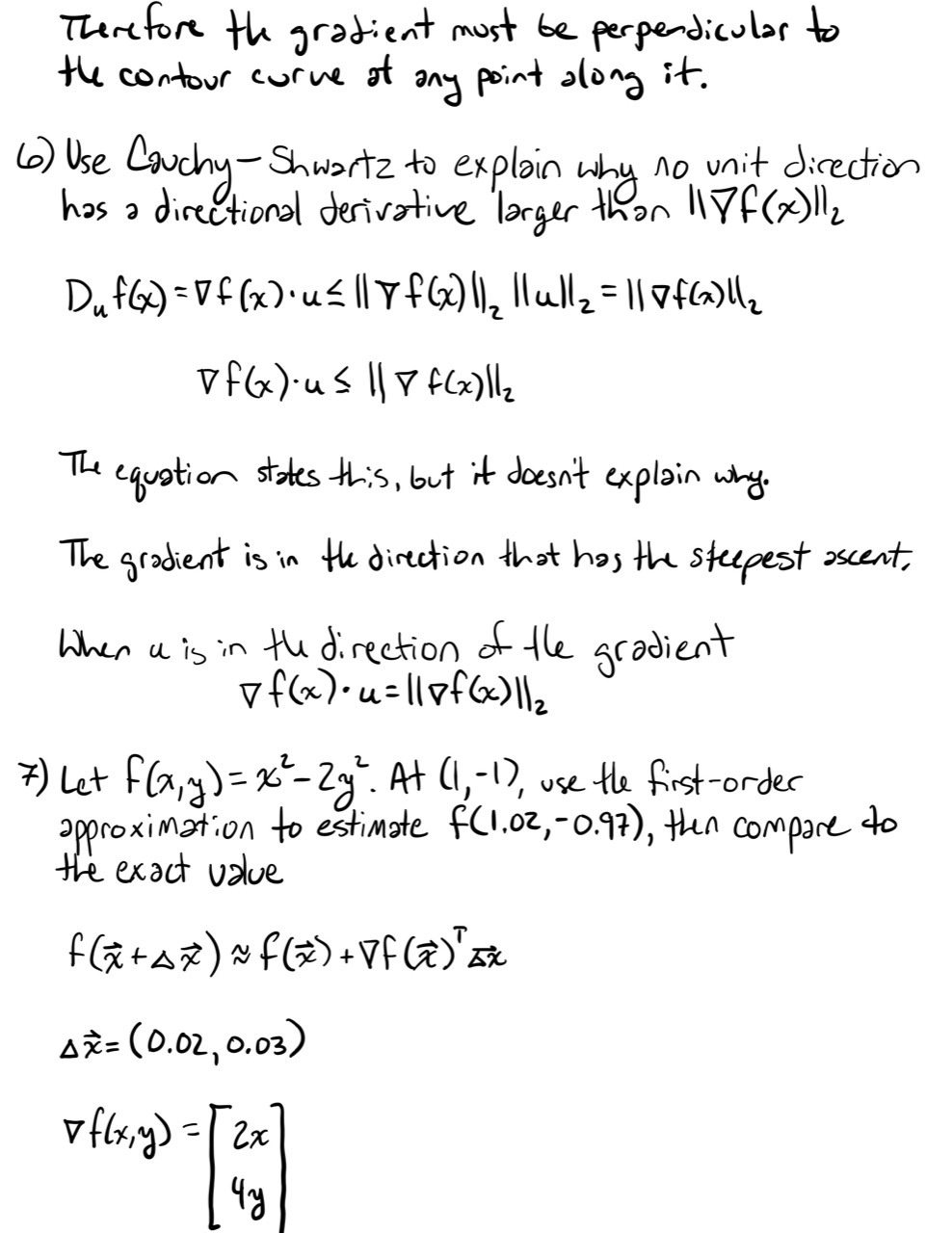
Explain geometrically why the gradient is perpendicular to a smooth contour line $f(x,y)=c$ .
Use Cauchy-Schwarz to explain why no unit direction has a directional derivative larger than $\lVert\nabla f(x)\rVert_2$ .
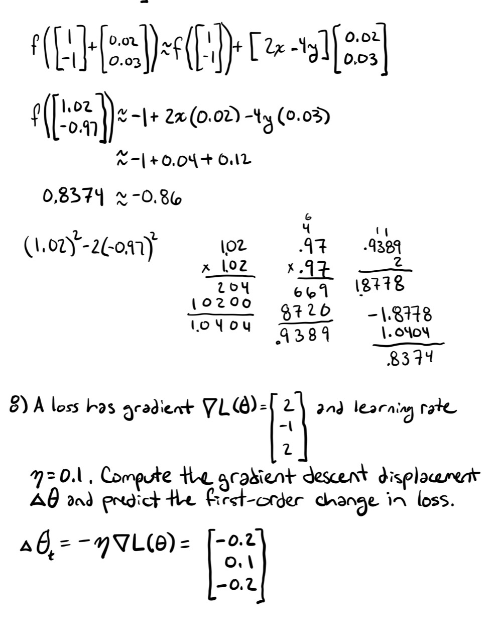
Let $f(x,y)=x^2+2y^2$ . At $(1,-1)$ , use the first-order approximation to estimate $f(1.02,-0.97)$ , then compare with the exact value.
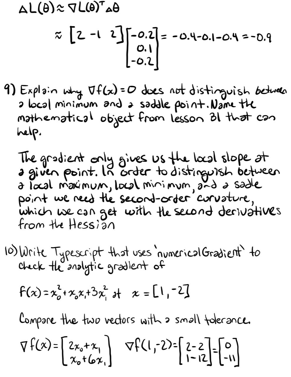
A loss has gradient $\nabla L(\theta)=[2,-1,2]^T$ and learning rate $\eta=0.1$ . Compute the gradient-descent displacement $\Delta\theta$ and the predicted first-order change in loss.
Explain why $\nabla f(x)=0$ does not distinguish a local minimum from a saddle point. Name the mathematical object from Lesson 31 that can help.
Write TypeScript that uses numericalGradient to check the analytic gradient of $f(x)=x_0^2+x_0x_1+3x_1^2$ at [1, -2]. Compare the two vectors with a small tolerance.
In your own words, distinguish the differential $df_x$ as a linear map from the gradient $\nabla f(x)$ as its Euclidean coordinate representation.

Summary

The gradient assembles every first partial derivative of a scalar field.
A directional derivative is the dot product $\nabla f(x)^Tu$ .
Among unit directions, the gradient points toward steepest local increase.
The negative gradient points toward steepest local decrease.
The gradient supplies the first-order approximation $\Delta f\approx\nabla f(x)^T\Delta x$ .
The differential is the local linear map; the Euclidean inner product represents it as a gradient vector.
Gradient descent uses this local information, while curvature limits how far a step can safely trust it.

Next Lesson

Lesson 36 generalizes from scalar outputs to vector outputs. The Jacobian collects the derivatives of every output with respect to every input and makes the local linear-map shape explicit.

Completed Exercises

Handwritten work submitted after completing this lesson.