Goal
Generalize the gradient from a function that returns one number to a function that returns a vector.
The result is the Jacobian: a matrix that answers
If the input moves a little, how does every output move?
Motivation
Lesson 35 studied a scalar field:
Its derivative maps an input displacement to one first-order output change. But most machine-learning systems contain intermediate functions with several outputs:
- a linear layer produces a vector of activations;
- a feature transform returns many features;
- a softmax maps a vector of logits to a vector of probabilities;
- a computation graph passes vector-valued state between operations.
For
the local derivative must turn an -dimensional input displacement into an -dimensional output displacement. A matrix has exactly that shape.
Intuition: A Tiny Linear Machine
A nonlinear function may bend and stretch space differently at different points. Near one chosen point, however, a differentiable function is approximately linear.
The Jacobian is the matrix for that local linear machine:
Read this from right to left:
- choose a small input motion ;
- apply the local matrix ;
- obtain the predicted output motion .
The Jacobian can change from point to point even though each individual Jacobian acts linearly on small displacements.
Notation / Symbol Table
| Symbol | Plain-English name | Shape and meaning |
|---|---|---|
| vector-valued function | Accepts inputs and returns outputs. | |
| input point | Point where the local derivative is evaluated. | |
| output component | The th scalar output of . | |
| Jacobian | matrix of output-by-input partial derivatives. | |
| input displacement | Small movement in input space. | |
| output displacement | First-order response in output space. | |
| input basis vector | Unit motion through input coordinate . |
The course uses the output-by-input convention:
Rows correspond to outputs. Columns correspond to inputs.
Formal Definition
Write the vector-valued function component by component:
Its Jacobian is:
The entry in row , column is:
Use the sentence output with respect to input to recover the order.
Shape Discipline
Before differentiating, write the function shape:
Then the Jacobian shape follows automatically:
This makes the local approximation type-check:
If those inner dimensions do not match, either the Jacobian convention or the multiplication order is wrong.
Worked Example: Two Inputs, Two Outputs
Let:
There are two outputs and two inputs, so the Jacobian is .
Differentiate the first output:
Differentiate the second output:
Transpose those output gradients into rows:
At :
Use The Jacobian For A Local Prediction
Suppose the input moves by:
Then:
Both outputs have zero first-order change in this direction at this point. That does not mean the nonlinear function is exactly constant; second-order terms may remain.
Indeed, the exact new input is :
The small discrepancy is the higher-order error that the first-order Jacobian approximation omits.
Reading Rows And Columns
The same Jacobian supports two complementary readings.
A Row Is One Output’s Gradient
Row contains the sensitivity of output to every input:
This is the output-centered view: choose one output and ask which inputs influence it.
A Column Is One Input Direction’s Effect
Column records how every output changes when only input moves:
This is the input-centered view: choose one coordinate motion and observe the complete output response.
Rows organize scalar sensitivities by output. Columns organize vector responses by input.
Gradients And Ordinary Derivatives Are Special Cases
The Jacobian unifies earlier derivative objects.
Scalar Output
For
the Jacobian has shape :
The course stores the gradient itself as an column vector, so its transpose is the scalar function’s Jacobian under the output-by-input convention.
Scalar Input
For
the Jacobian has shape . It is the column of ordinary derivatives of every output with respect to the one input.
Scalar Input And Scalar Output
For
the Jacobian is : the familiar derivative .
Linear Maps Have Constant Jacobians
Consider an affine function:
where .
Its Jacobian is:
The bias disappears because a constant does not change with the input. The Jacobian is the same everywhere because the linear part does not bend.
For a nonlinear function, depends on . The Jacobian is the point-dependent matrix that locally plays the role of .
Connection To The Chain Rule
Suppose:
and
Their composition has shape:
The Jacobian shapes predict the chain rule:
The order matches function composition: acts first on the input, and acts second on the intermediate output.
Lesson 37 develops this multiplication rule through computation graphs and backpropagation.
Connection To Programming
A vector field accepts a vector and returns a vector:
type VectorField = (x: readonly number[]) => readonly number[];A centered finite-difference Jacobian can perturb each input coordinate and measure every output response:
function numericalJacobian(
  f: VectorField,
  at: readonly number[],
  h = 1e-5,
): number[][] {
  const outputSize = f(at).length;
  const columns = at.map((_, coordinate) => {
    const plus = at.map((value, index) =>
      index === coordinate ? value + h : value,
    );
    const minus = at.map((value, index) =>
      index === coordinate ? value - h : value,
    );
    const fPlus = f(plus);
    const fMinus = f(minus);

    return fPlus.map((value, output) =>
      (value - fMinus[output]) / (2 * h),
    );
  });

  return Array.from({ length: outputSize }, (_, output) =>
    columns.map((column) => column[output]),
  );
}
The perturbation loop naturally produces columns: each input coordinate is changed once, and all output responses are observed. The final transformation arranges those columns into the course’s output-by-input matrix convention.
Common Mistakes
Swapping Rows And Columns
Write first. Under this lesson’s convention, the Jacobian is : outputs by inputs.
Forgetting That Every Output Is Differentiated
A gradient handles one scalar output. A Jacobian contains one transposed output gradient per row.
Treating The Jacobian As Globally Linear
is a local linear approximation at . For a nonlinear , the matrix changes with the evaluation point.
Multiplying In The Wrong Order
The local input displacement is a column vector, so use . Shape checking exposes the reversed order.
Confusing A Zero First-Order Change With Exact Constancy
If , the chosen direction has no first-order effect at that point. Higher-order changes may still occur.
Exercises
-
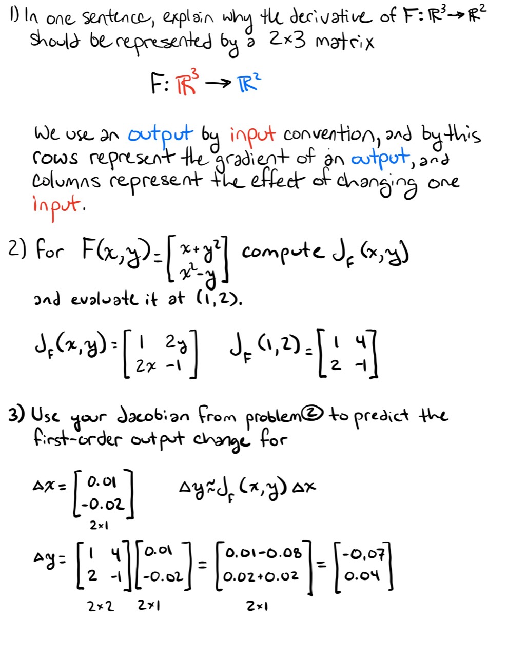
In one sentence, explain why the derivative of should be represented by a matrix.
-
For
compute and evaluate it at .
-
Use your Jacobian from Problem 2 to predict the first-order output change for
-
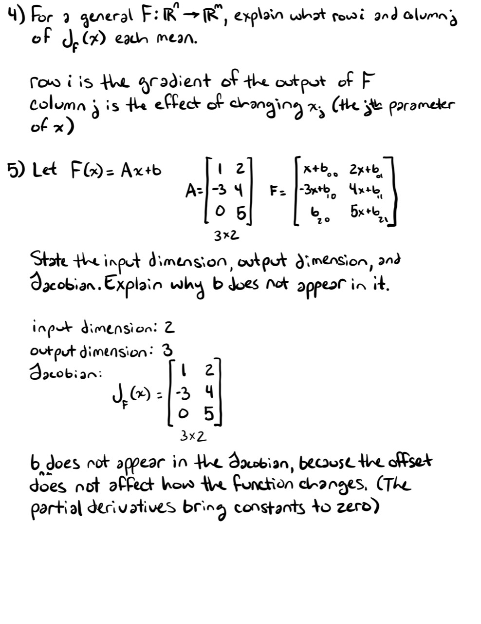
For a general , explain what row and column of each mean.
-
Let
State the input dimension, output dimension, and Jacobian. Explain why does not appear in it.
-
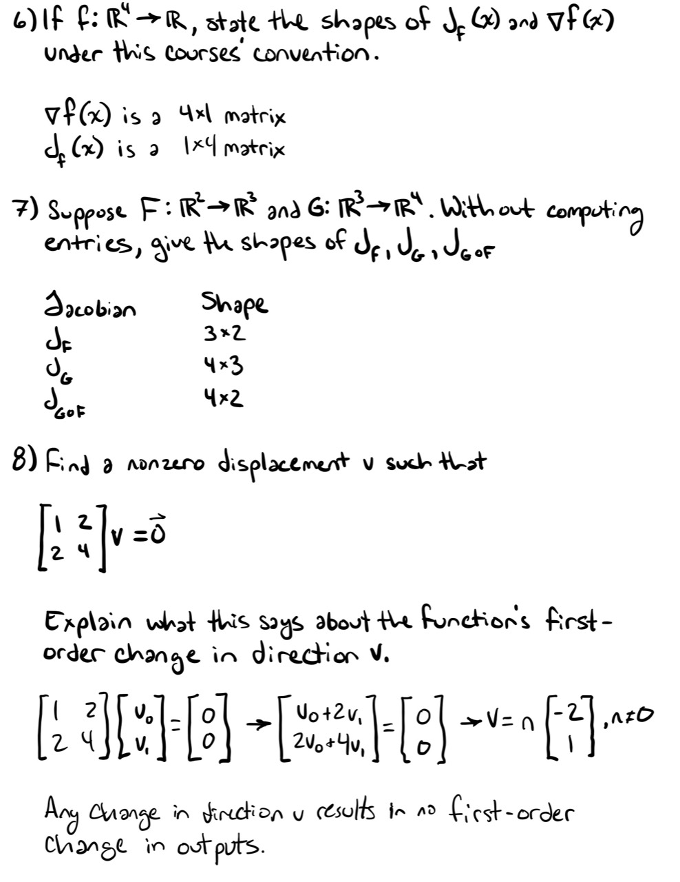
If , state the shapes of and under this course’s convention, and write their relationship.
-
Suppose and . Without computing entries, give the shapes of , , and , then write the only multiplication order that type-checks.
-
Find a nonzero displacement such that
Explain what this says about the function’s first-order change in direction .
-
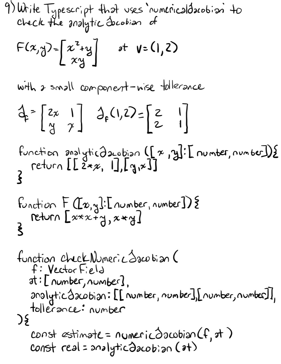
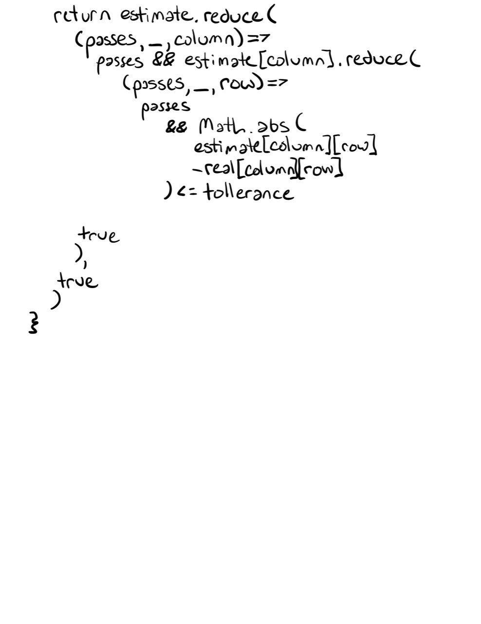
Write TypeScript that uses
numericalJacobianto check the analytic Jacobian ofat
[1, 2]with a small componentwise tolerance. -
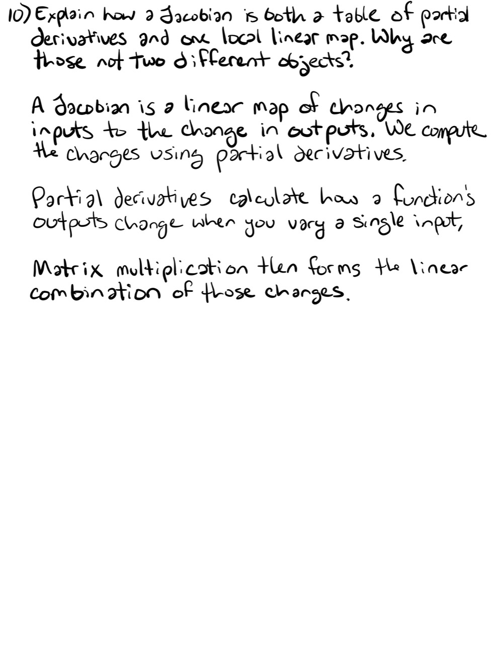
In your own words, explain how a Jacobian is both a table of partial derivatives and one local linear map. Why are those not two different objects?
Summary
- The Jacobian is the derivative of a vector-valued function.
- For , the course uses .
- Entry is the sensitivity of output to input .
- Rows are transposed output gradients; columns are complete responses to input-coordinate motion.
- The local approximation is .
- A scalar function’s Jacobian is the transpose of its column gradient.
- Affine maps have constant Jacobians equal to their linear matrices.
- Jacobian multiplication is the shape-disciplined form of the chain rule.
Next Lesson
Lesson 37 uses Jacobians to differentiate compositions. Computation graphs make the chain rule operational: local derivative maps multiply in forward composition order, while backpropagation efficiently moves sensitivity information backward.
Completed Exercises
Handwritten work submitted after completing this lesson.