Goal
Turn the chain rule from a formula about nested functions into an algorithm for differentiating a program.
The central idea is:
A large derivative is assembled from small local derivatives, following the same dependency structure as the original computation.
Why Composition Creates A New Problem
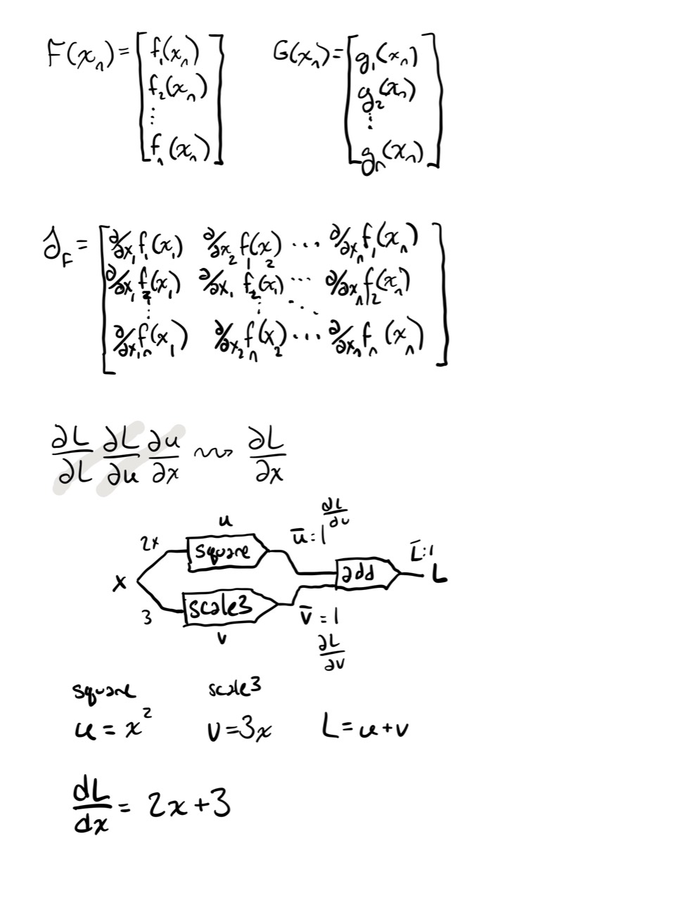
Lesson 36 described one function near one point with one Jacobian:
Real models are compositions. An input becomes a linear transformation, then an activation, then another transformation, and eventually a scalar loss. Writing the entire model as one expanded formula would hide the reusable structure and create a large bookkeeping problem.
A computation graph keeps that structure explicit:
input -> intermediate values -> prediction -> lossEach node performs a small operation. The chain rule explains how their local derivatives combine.
The Invariant: Derivatives Must Connect Compatible Spaces
Suppose:
and:
The composition is:
Its derivative must map an -dimensional input displacement to a -dimensional output displacement. The Jacobian chain rule is:
The shapes force the order:
This is the same composition rule as matrix transformations. acts first, so its Jacobian is closest to the input displacement on the right.
Notation / Symbol Table
| Symbol | Plain-English name | Meaning |
|---|---|---|
| graph input | Value supplied to the first operation. | |
| intermediate values | Named results stored by graph nodes. | |
| scalar loss | Final scalar output whose sensitivities we want. | |
| composition | Apply first, then apply . | |
| local Jacobian of | Maps a small displacement through the node. | |
| local scalar derivative | Sensitivity of child value to parent value . | |
| reverse sensitivity | Sensitivity of the final loss to intermediate value . | |
| input sensitivity | Gradient of the final loss with respect to the graph input. |
The bar in does not mean an average. In this lesson it is compact notation for the derivative of the final scalar loss with respect to .
First Example: A Scalar Chain
Let:
The graph is:
x --square--> u --scale and shift--> LThe local derivatives are:
The chain rule multiplies them:
At , the forward values are:
The backward sensitivities are:
The forward pass computes values. The backward pass computes how the final loss depends on those values.
Why The Backward Pass Starts With One
Every reverse pass begins at the final scalar output with:
This is not an arbitrary initialization. A quantity changes one-for-one with itself. That unit sensitivity seeds the repeated chain-rule multiplications.
A Computation Graph Is A Factorization
Consider:
Factor it into named operations:
The graph is:
x --\
     multiply -> u -> add 1 -> v -> square -> L
y --/
At , the forward pass gives:
Now record only the local derivatives:
Propagate backward:
Therefore:
The graph avoided expanding the whole expression. Each node needed only its own operation, stored forward values, and incoming sensitivity.
Branching Means Addition
Multiplication handles consecutive links along one path. Addition handles several paths from the same variable to the output.
Let:
The input influences along two paths:
       -> square -> u --\
x ---->              add -> L
       -> scale  -> v --/
The total derivative is the sum of both path contributions:
Since both addition-node derivatives are :
This yields the operational rule:
Multiply local derivatives along a path. Add contributions from different paths that meet at the same value.
Failing to add at a branch is one of the most common computation-graph mistakes.
Vector Composition
The same rule works when intermediate values are vectors.
Let:
Then:
Their product is:
Because is scalar-valued, this result is the transpose of its column gradient:
This transposed form is important in machine learning. It says that an output gradient can be pulled backward through by multiplying with .
A Concrete Vector Example
Define:
The local Jacobians are:
and:
At , the intermediate value is:
Therefore:
Compose them:
Thus:
The shapes are not decoration. They tell us which maps can be composed and in what order.
Forward Mode And Reverse Mode
There are two natural ways to apply the chain rule without constructing every full derivative matrix.
Forward Accumulation
Start with an input direction and push its effect forward:
This computes a Jacobian-vector product:
It efficiently answers: How does this chosen input direction affect every output?
Reverse Accumulation
Start with sensitivity at a scalar loss and pull it backward:
This computes a vector-Jacobian product, usually represented with column gradients through the transpose.
It efficiently answers: How does the one final loss depend on every earlier input or parameter?
Machine learning commonly has millions of parameters but one scalar loss. That shape makes reverse accumulation especially valuable: one backward sweep can produce sensitivities for every parameter.
This Is The Foundation Of Backpropagation
Backpropagation is not a different derivative rule. It is reverse-mode chain-rule accumulation specialized to layered models and scalar losses.
This lesson focuses on the calculus and graph bookkeeping. Lesson 43 will apply the same mechanism to neural-network parameters, activations, and layers.
Connection To Programming
Here is the earlier branching example encoded as an explicit forward pass and backward pass:
type ForwardState = Readonly<{
  loss: number;
  scaled: number;
  squared: number;
  x: number;
}>;

function forward(x: number): ForwardState {
  const squared = x * x;
  const scaled = 3 * x;
  const loss = squared + scaled;

  return { loss, scaled, squared, x };
}

function backward(state: ForwardState): number {
  const lossSensitivity = 1;
  const squaredSensitivity = lossSensitivity * 1;
  const scaledSensitivity = lossSensitivity * 1;

  const fromSquared = squaredSensitivity * (2 * state.x);
  const fromScaled = scaledSensitivity * 3;

  return fromSquared + fromScaled;
}

const state = forward(2);
const derivative = backward(state);

console.assert(state.loss === 10);
console.assert(derivative === 7);
Notice the software structure:
- The forward pass stores values needed by local derivative formulas.
- The backward pass receives a sensitivity from each child.
- Each edge multiplies by one local derivative.
- Contributions are added when they reach a shared parent.
A full automatic-differentiation engine generalizes this pattern by storing operations and their local backward rules dynamically.
Common Mistakes
Reversing The Jacobian Product
For , write the displacement flow:
Therefore is closest to on the right:
Evaluating A Local Derivative At The Wrong Value
must be evaluated at the intermediate value , not at the original input unless those happen to be the same type and value.
Multiplying Across Branches Instead Of Adding
Consecutive edges multiply. Alternative paths add. A reused value can receive several valid sensitivity contributions.
Mixing Forward Values With Backward Sensitivities
is an intermediate value. is a sensitivity. They may have compatible shapes, but they represent different things.
Materializing A Full Jacobian Unnecessarily
If the goal is only a directional effect or scalar-loss gradient, Jacobian-vector and vector-Jacobian products can apply the local map without storing every entry of a large Jacobian.
Exercises
-
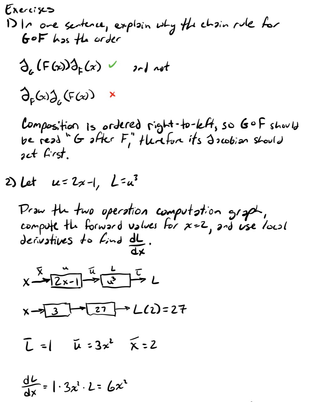
In one sentence, explain why the chain rule for has the order rather than .
-
Let:
Draw the two-operation computation graph, compute the forward values at , and use local derivatives to find .
-
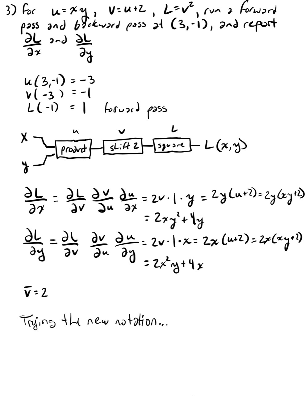
For:
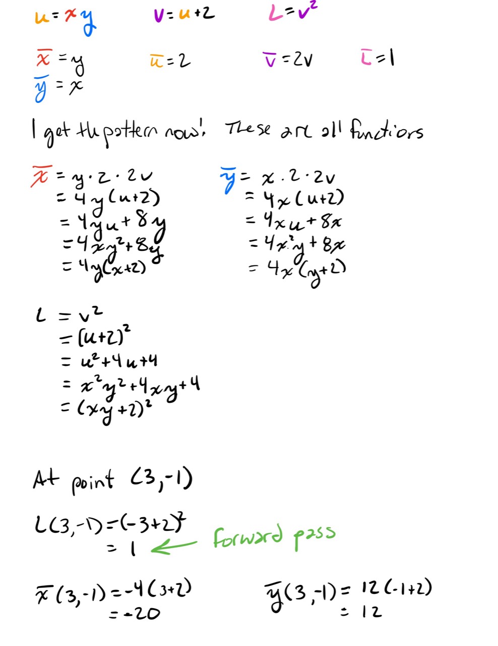
run a forward and backward pass at and report and .
-
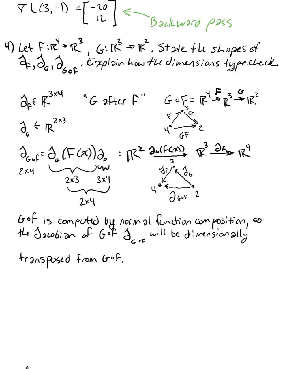
Let and . State the shapes of , , and . Explain how the dimensions type-check.
-
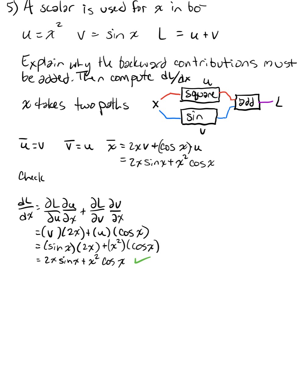
A scalar is used in both:
Explain why the backward contributions to must be added, then compute .
-
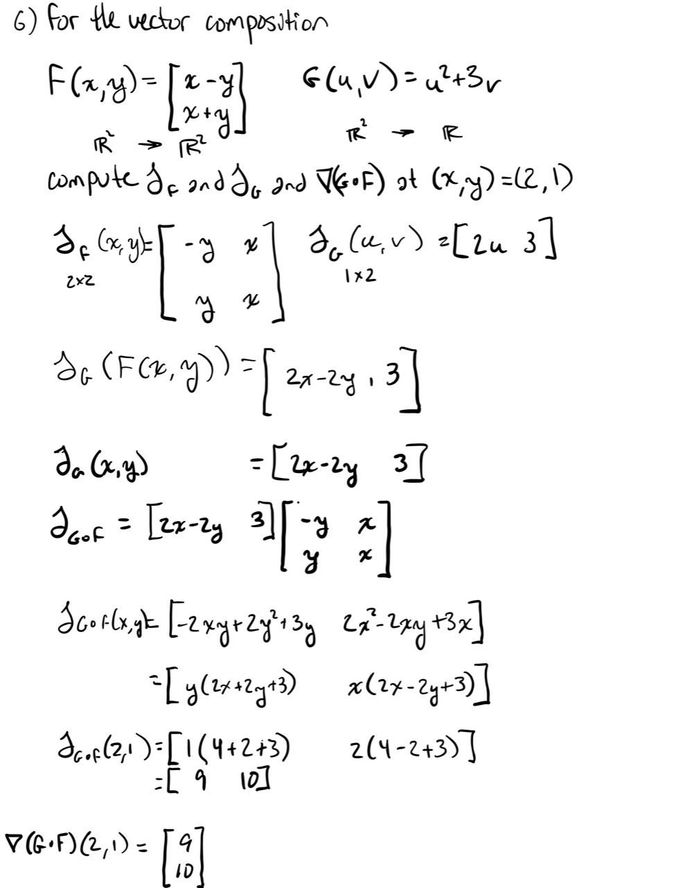
For the vector composition:
compute , , and at using Jacobian multiplication.
-
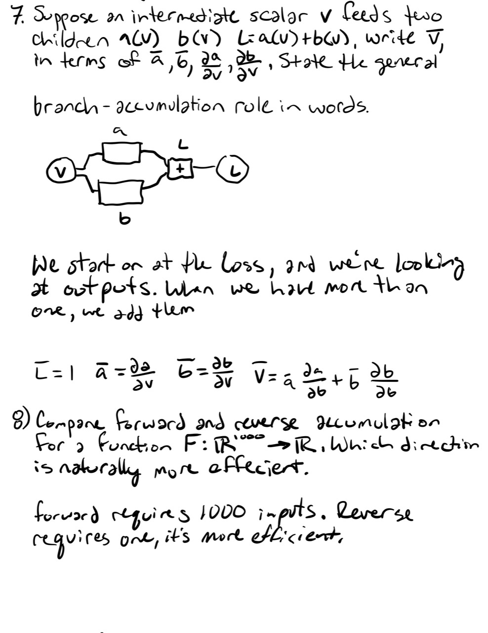
Suppose an intermediate scalar feeds two children and , and . Write in terms of , , , and . State the general branch-accumulation rule in words.
-
Compare forward and reverse accumulation for a function . Which direction is naturally efficient for computing the full gradient of the scalar output, and why?
-
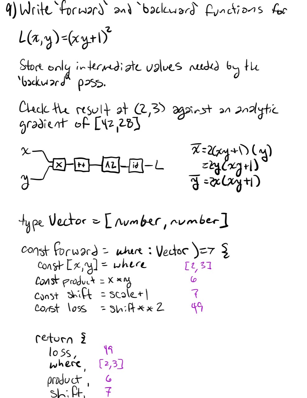
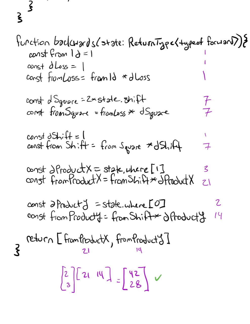
Write TypeScript
forwardandbackwardfunctions for:Store only the intermediate values needed by the backward pass. Check the result at against the analytic gradient .
-
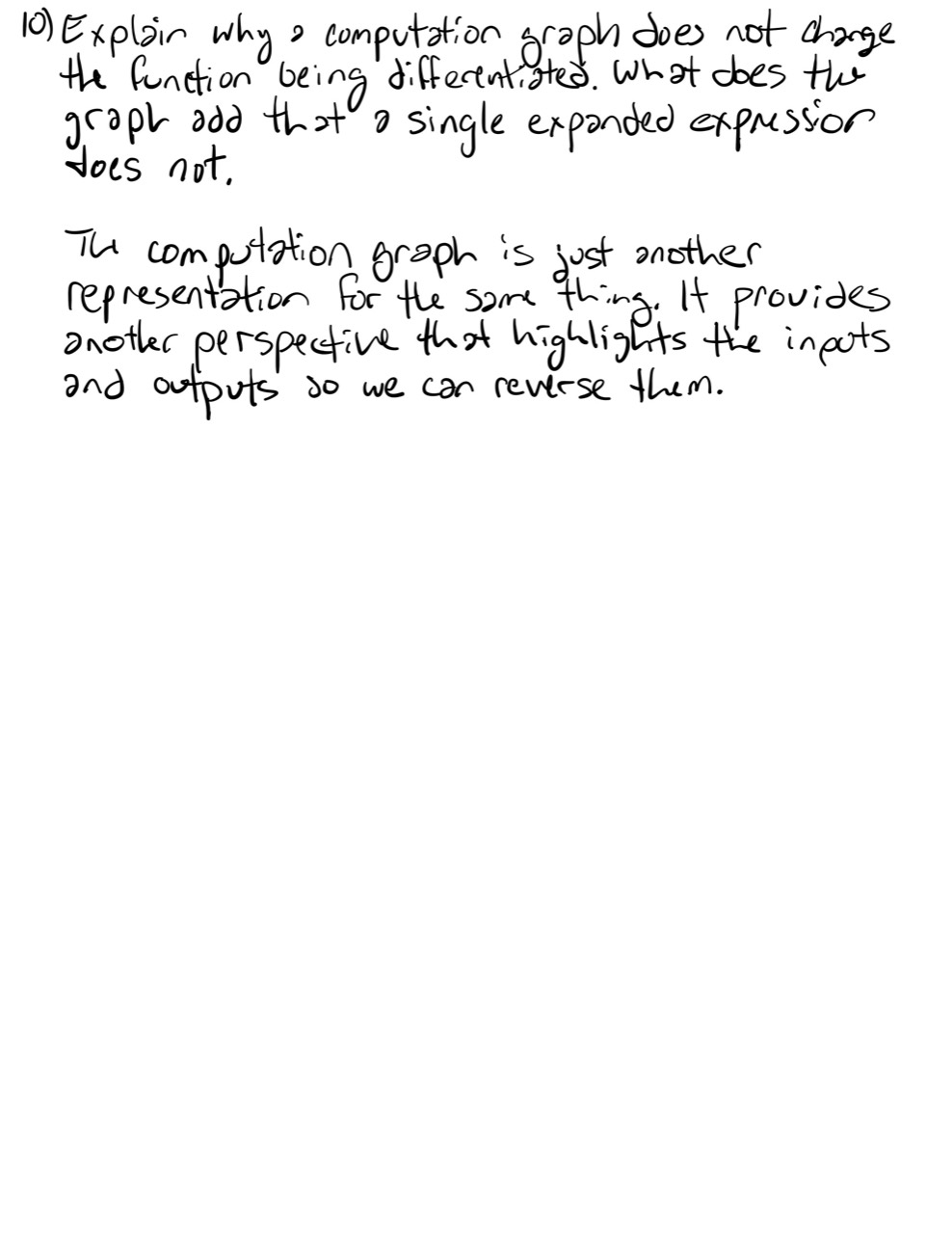
In your own words, explain why a computation graph does not change the function being differentiated. What does the graph add that the single expanded expression does not?
Practice 37.1: Local Derivatives And Branch Accumulation
This is a short correction checkpoint, not a new lesson. Work it on paper without expanding the full functions first. For every computation, write the forward values separately from the backward sensitivities.
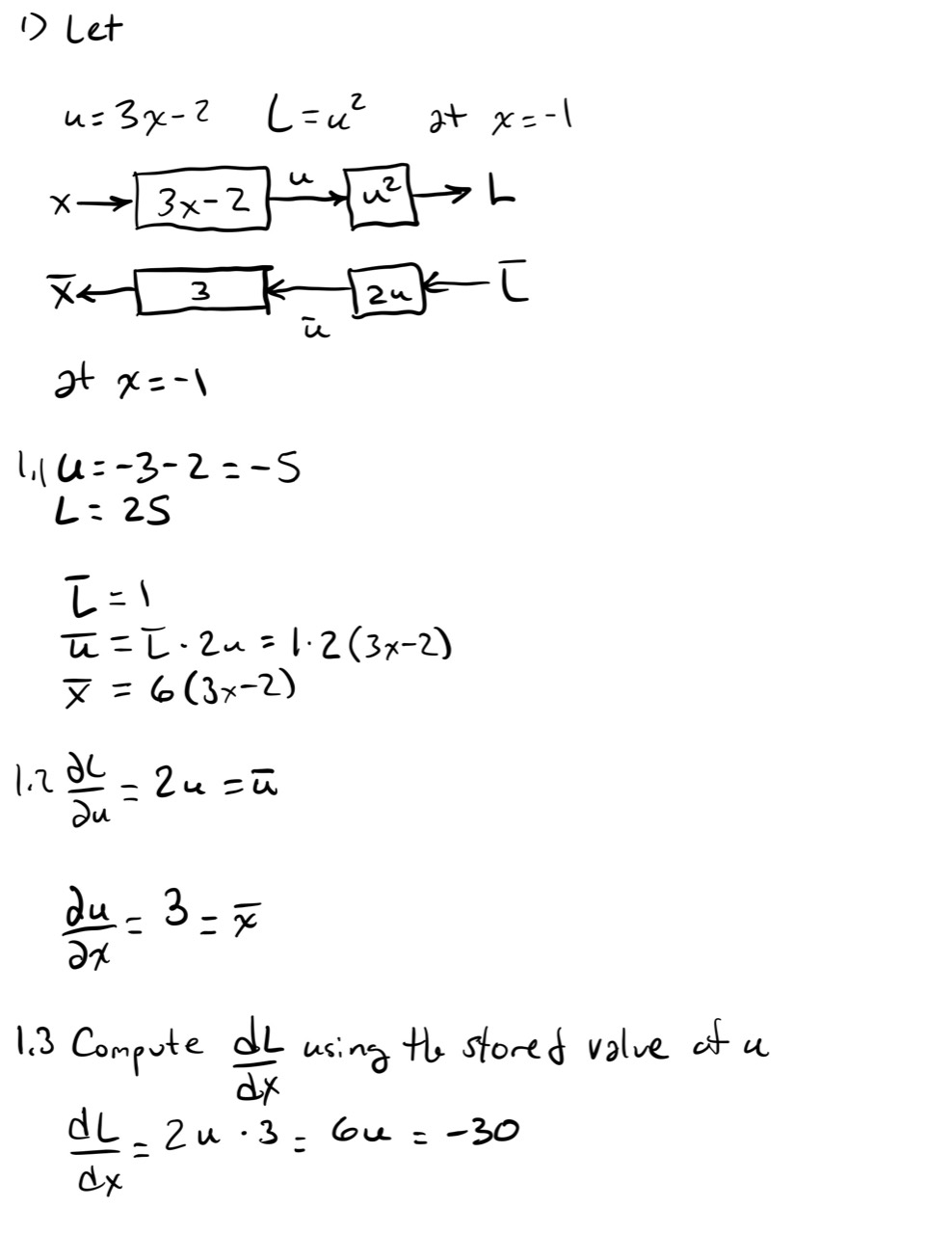
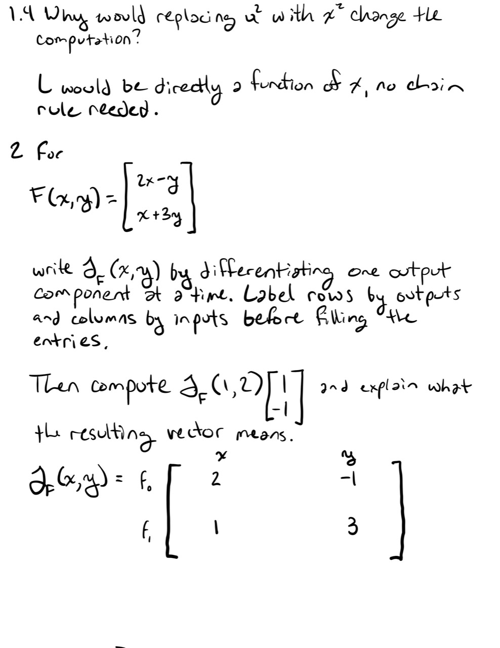
1. Local Values Stay Local
Let:
At :
- Compute the forward values and .
- Write the local derivatives and .
- Compute using the stored value of .
- In one sentence, explain why replacing with would change the computation.
2. Follow The Actual Operations
For:
write by differentiating one output component at a time. Label rows by outputs and columns by inputs before filling in the entries.
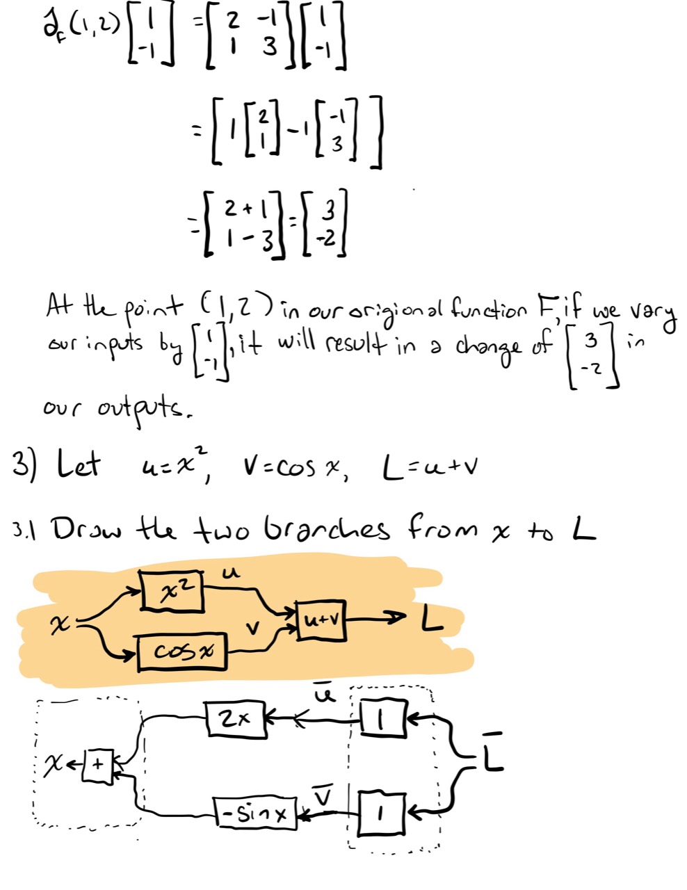
Then compute:
and explain what the resulting vector means.
3. Addition At A Branch
Let:
- Draw the two branches from to .
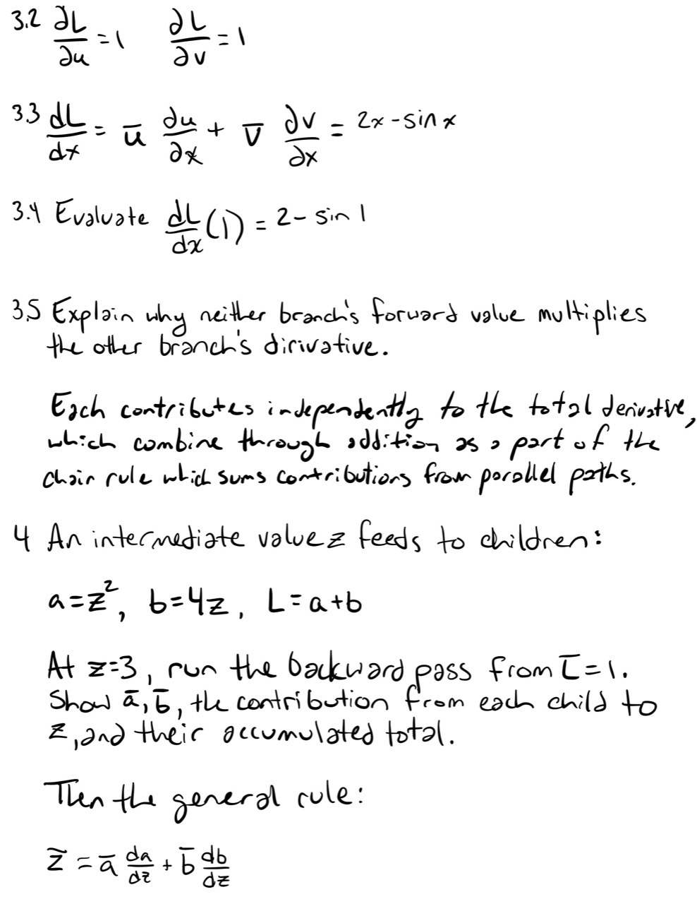
- Write the local derivatives at the final addition node.
- Compute symbolically.
- Evaluate it at .
- Explain why neither branch’s forward value multiplies the other branch’s derivative.
4. Accumulate Child Contributions
An intermediate value feeds two children:
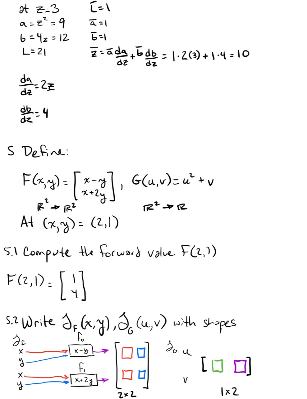
At , run the backward pass from . Show , , the contribution from each child to , and their accumulated total.
Then write the general rule:
using , , , and .
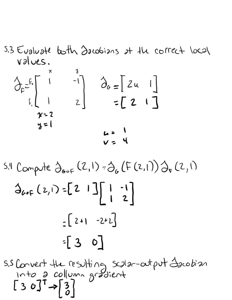
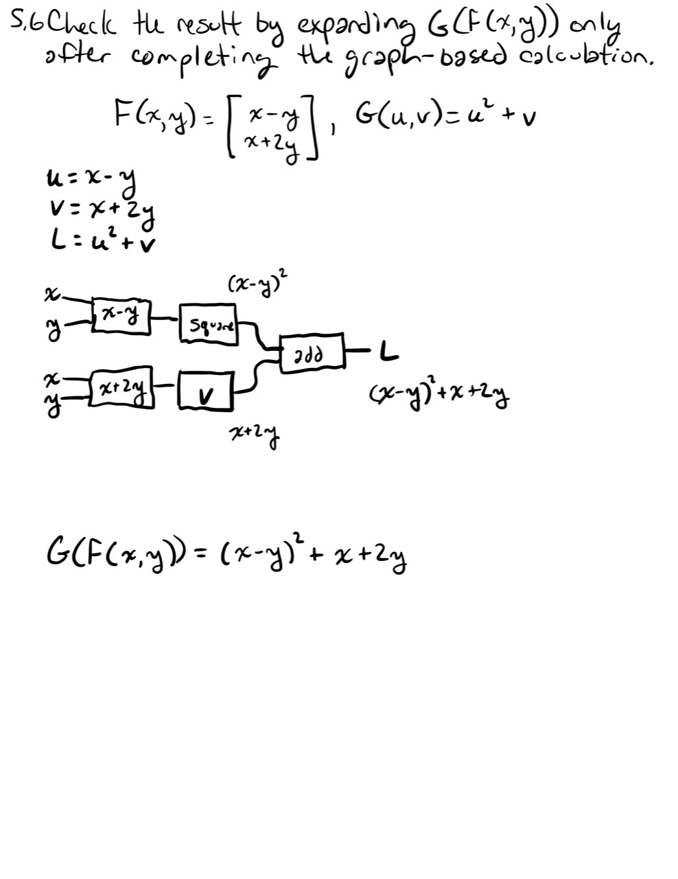
5. One Complete Composition
Define:
At :
- Compute the forward value .
- Write and with shapes.
- Evaluate both Jacobians at the correct local values.
- Compute .
- Convert the resulting scalar-output Jacobian into a column gradient.
- Check the result by expanding only after completing the graph-based calculation.
Readiness Check
Lesson 37 is ready to close when the work consistently shows all four habits:
- Local derivatives are evaluated using the stored value at their own node.
- The derivative matches the operation actually written in each node or component.
- Derivatives multiply along one path.
- Contributions add when several paths return to the same parent.
Summary
- A computation graph factors a function into small operations and explicit dependencies.
- The chain rule composes local derivative maps.
- For , the Jacobian is .
- The forward pass computes and stores values.
- The backward pass propagates final-output sensitivities through local derivatives.
- Local derivatives multiply along one path and contributions add across multiple paths.
- Forward accumulation pushes a chosen input direction toward outputs.
- Reverse accumulation pulls a scalar loss sensitivity back toward every input and parameter.
- Backpropagation is reverse chain-rule accumulation applied to neural networks.
Next Lesson
Lesson 38 makes matrix-calculus layout conventions explicit. We will use shape checking to distinguish gradients with respect to vectors and matrices, translate between common notation conventions, and derive reusable identities without relying on memorized formula tables.
Completed Exercises
Handwritten work submitted after completing this lesson.