Lesson 38: Matrix Calculus Notation

Goal

Make matrix-calculus notation behave like a type system: the input and output spaces determine the derivative’s job, and its shape exposes many mistakes before any algebra is finished.

The central rule is:

Decide what linear map the derivative must represent, write its shape, and only then choose notation for it.

A Short Bridge From Computation Graphs

Before adding new notation, separate three operations that looked similar in the previous lesson.

Evaluate Local Derivatives At Local Values

If:

u=2x-1, \qquad L=u^3,

then:

\frac{dL}{dx} = \frac{\partial L}{\partial u} \frac{\partial u}{\partial x} =3u^2(2).

At $x=2$ , the stored intermediate value is $u=3$ , so:

\frac{dL}{dx}=3(3)^2(2)=54.

The square belongs to $u$ , not to the original input $x$ .

Differentiate The Operation That Is Actually Present

If:

L=x^2+\sin x,

the final operation is addition. Its local derivatives are both $1$ , so the two paths contribute:

\frac{dL}{dx}=2x+\cos x.

Factors such as $\sin x$ and $x^2$ would appear if the final operation were multiplication. A graph prevents that accidental change of program.

Build Jacobians From Component Functions

For:

F(x,y)= \begin{bmatrix} x-y\\ x+y \end{bmatrix},

differentiate each output with respect to each input:

J_F(x,y)= \begin{bmatrix} 1 & -1\\ 1 & 1 \end{bmatrix}.

Do not infer the derivative from the visual presence of two variables. Read the actual addition, subtraction, multiplication, or other operation in each component.

These are the same habits matrix calculus needs: local values, actual operations, and explicit shapes.

Notation / Symbol Table

Symbol	Shape	Meaning
$x\in\mathbb R^n$	$n\times1$	Column-vector input.
$F(x)\in\mathbb R^m$	$m\times1$	Column-vector output.
$J_F(x)$	$m\times n$	Output-by-input Jacobian.
$\nabla_x f$	$n\times1$	Column gradient of scalar $f$ with respect to $x$ .
$dx$	$n\times1$	Small input displacement.
$df$	scalar	First-order change in a scalar function.
$X\in\mathbb R^{p\times q}$	$p\times q$	Matrix input.
$\nabla_X f$	$p\times q$	Matrix gradient paired with $dX$ .
$\operatorname{tr}(A)$	scalar	Sum of diagonal entries of square $A$ .
$\langle A,B\rangle_F$	scalar	Frobenius inner product $\operatorname{tr}(A^TB)$ .

Derivatives Are Linear Maps Before They Are Arrays

Let:

F:\mathbb R^n\to\mathbb R^m.

Near $x$ , the derivative consumes an input displacement and produces an output displacement:

dF=J_F(x)\,dx.

The shapes must be:

\underbrace{dF}_{m\times1} = \underbrace{J_F(x)}_{m\times n} \underbrace{dx}_{n\times1}.

That requirement is more fundamental than the notation $J_F$ . Any notation convention must still encode this same local linear map.

For a scalar function:

f:\mathbb R^n\to\mathbb R,

the differential is:

df=(\nabla_x f)^Tdx.

Again the shapes explain the transpose:

\underbrace{df}_{1\times1} = \underbrace{(\nabla_x f)^T}_{1\times n} \underbrace{dx}_{n\times1}.

Two Layout Families

Different books arrange the same partial derivatives differently. Let $F:\mathbb R^n\to\mathbb R^m$ .

Numerator Layout

Numerator layout places output coordinates in rows and input coordinates in columns:

\frac{\partial F}{\partial x} = \begin{bmatrix} \frac{\partial F_1}{\partial x_1} & \cdots & \frac{\partial F_1}{\partial x_n}\\ \vdots & \ddots & \vdots\\ \frac{\partial F_m}{\partial x_1} & \cdots & \frac{\partial F_m}{\partial x_n} \end{bmatrix} \in\mathbb R^{m\times n}.

This is the Jacobian convention used by this course because it acts directly in:

dF=J_F\,dx.

For scalar $f$ , the same layout produces a $1\times n$ row derivative.

Denominator Layout

Denominator layout transposes that array:

\left(\frac{\partial F}{\partial x}\right)_{\text{denominator}} \in\mathbb R^{n\times m}.

For scalar $f$ , this produces an $n\times1$ column—the same shape commonly assigned to $\nabla_x f$ .

The Course Convention

This course uses a practical hybrid that is common in machine learning:

Vector-output derivatives use the output-by-input Jacobian $J_F\in\mathbb R^{m\times n}$ .
Scalar-output derivatives use the column gradient $\nabla_x f\in\mathbb R^{n\times1}$ .
They are related by $J_f=(\nabla_x f)^T$ .

The names “numerator” and “denominator” are less important than declaring the shape. When reading another source, ask:

Are vectors columns or rows?
What shape does it assign to a scalar-by-vector derivative?
Does its chain rule multiply on the left or the right?
Is its displayed object a Jacobian, a gradient, or a transpose of one?

Shape Checking As A Compiler

Suppose:

x\in\mathbb R^n, \qquad A\in\mathbb R^{m\times n}, \qquad y=Ax+b\in\mathbb R^m.

The derivative with respect to $x$ must map an $n$ -vector displacement to an $m$ -vector displacement, so:

J_y(x)=A\in\mathbb R^{m\times n}.

Now let $f:\mathbb R^m\to\mathbb R$ . The chain rule in column-gradient form is:

\nabla_x(f\circ y) = J_y(x)^T\nabla_y f =A^T\nabla_y f.

The shape check is:

\underbrace{\nabla_x f}_{n\times1} = \underbrace{A^T}_{n\times m} \underbrace{\nabla_y f}_{m\times1}.

This is exactly the vector form of a backward pass.

Differentials: A Convention-Resistant Method

Differentials let us derive gradients by matching a standard shape instead of recalling a formula.

For a vector input, arrange the result as:

df=(\nabla_x f)^Tdx.

Whatever multiplies $dx$ as a row is $(\nabla_x f)^T$ .

Linear Form

Let:

f(x)=a^Tx.

Then:

df=a^Tdx.

Matching the standard form gives:

\nabla_x f=a.

Quadratic Form

Let:

f(x)=x^TAx.

Apply the product rule:

df=(dx)^TAx+x^TA(dx).

The first scalar term can be transposed without changing its value:

(dx)^TAx=x^TA^Tdx.

Therefore:

df=x^T(A^T+A)dx,

so:

\nabla_x f=(A+A^T)x.

If $A$ is symmetric, this reduces to:

\nabla_x f=2Ax.

The familiar $2Ax$ formula requires symmetry. Shape checking alone cannot supply that assumption; it must be stated.

A Core ML Identity: Squared Error

Let:

r=Ax-b, \qquad L(x)=\lVert r\rVert^2=r^Tr.

First differentiate the residual:

dr=A\,dx.

Then differentiate the loss:

dL=2r^Tdr.

Substitute the local differential:

dL=2r^TA\,dx.

Match $dL=(\nabla_xL)^Tdx$ :

\nabla_xL=2A^Tr=2A^T(Ax-b).

The transpose is not a memorized decoration. It is forced when the row $2r^TA$ is converted into a column gradient.

Gradients With Respect To Matrices

Suppose a scalar function depends on a matrix:

f:\mathbb R^{p\times q}\to\mathbb R.

We define $\nabla_X f$ to have the same shape as $X$ and pair it with $dX$ using the Frobenius inner product:

df = \langle \nabla_X f,dX\rangle_F = \operatorname{tr}\left((\nabla_X f)^T dX\right).

This is the matrix analogue of $df=(\nabla_x f)^Tdx$ .

Trace Linear Form

Let:

f(X)=\operatorname{tr}(A^TX),

where $A$ and $X$ have the same shape. Then:

df=\operatorname{tr}(A^T dX).

Matching the standard matrix differential gives:

\nabla_X f=A.

The trace turns an entrywise sum into compact linear-algebra notation:

\operatorname{tr}(A^TX)=\sum_{i,j}A_{ij}X_{ij}.

Derivative Identity Ledger

These identities should be reconstructible from differentials and shapes:

Function	Gradient or Jacobian	Required assumptions
$y=Ax+b$	$J_y=A$	$A$ is constant.
$f=a^Tx$	$\nabla_x f=a$	$a$ is constant.
$f=x^TAx$	$\nabla_x f=(A+A^T)x$	$A$ is constant.
$f=x^TAx$	$\nabla_x f=2Ax$	$A$ is constant and symmetric.
$L=\lVert Ax-b\rVert^2$	$\nabla_xL=2A^T(Ax-b)$	$A$ and $b$ are constant.
$f(X)=\operatorname{tr}(A^TX)$	$\nabla_Xf=A$	$A$ is constant and has the same shape as $X$ .

Use this table as a checksum, not as a substitute for the derivations.

Reading A Paper Without Inheriting Its Convention Blindly

Suppose a paper writes:

\frac{\partial L}{\partial x}=g.

That line alone does not reveal whether $g$ is a row or column. Recover its meaning from use:

If the paper writes $dL=g\,dx$ , then $g$ acts like a row derivative.
If it writes $dL=g^Tdx$ , then $g$ acts like a column gradient.
If an update is $x\leftarrow x-\eta g$ , then $g$ must have the same shape as $x$ .
If a chain rule seems reversed, check whether every derivative array has been transposed by the source’s layout convention.

The invariant is the linear map and the scalar pairing, not the typography.

Connection To Programming

A lightweight shape ledger makes the convention explicit in code review:

type Shape = readonly [rows: number, columns: number];

type TypedValue = Readonly<{
  name: string;
  shape: Shape;
}>;

const canMultiply = (
  left: TypedValue,
  right: TypedValue,
): boolean => left.shape[1] === right.shape[0];

const jacobian: TypedValue = { name: 'J_F', shape: [3, 2] };
const displacement: TypedValue = { name: 'dx', shape: [2, 1] };

console.assert(canMultiply(jacobian, displacement));

Real tensor libraries carry richer shape information, but the mathematical habit is the same: reject incompatible compositions early.

Common Mistakes

Calling Every Derivative A Gradient

A gradient is naturally associated with a scalar output. A vector-valued function has a Jacobian or another explicitly declared derivative map.

Copying A Formula Without Its Convention

Two sources may display transposed arrays while representing the same derivative. Record vector orientation and expected shape before comparing formulas.

Losing A Transpose In A Backward Pass

Forward displacements use $dF=J_Fdx$ . Backward column gradients use $\nabla_xL=J_F^T\nabla_FL$ .

Using The Symmetric Quadratic Identity Without Symmetry

$\nabla_x(x^TAx)=2Ax$ only when $A=A^T$ . The general result is $(A+A^T)x$ .

Treating Shape Checking As A Complete Proof

Several wrong formulas can have the right shape. Shape checking rejects many errors, but component definitions, local values, and algebra still matter.

Exercises

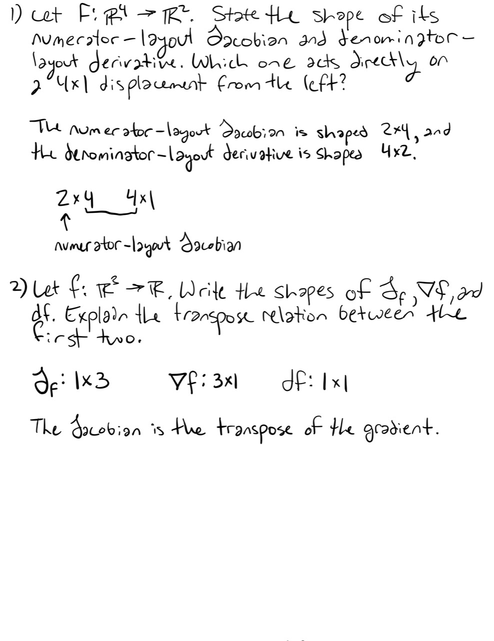
Let $F:\mathbb R^4\to\mathbb R^2$ . State the shape of its numerator-layout Jacobian and denominator-layout derivative. Which one acts directly on a $4\times1$ displacement from the left?
Let $f:\mathbb R^3\to\mathbb R$ . Write the shapes of $J_f$ , $\nabla f$ , and $df$ . Explain the transpose relation between the first two.
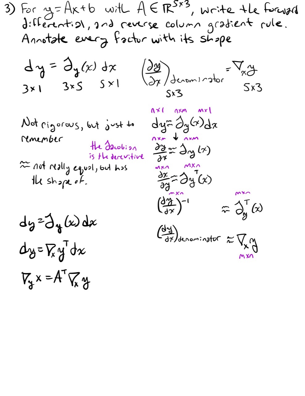
For $y=Ax+b$ with $A\in\mathbb R^{5\times3}$ , write the forward differential and the reverse column-gradient rule. Annotate every factor with its shape.
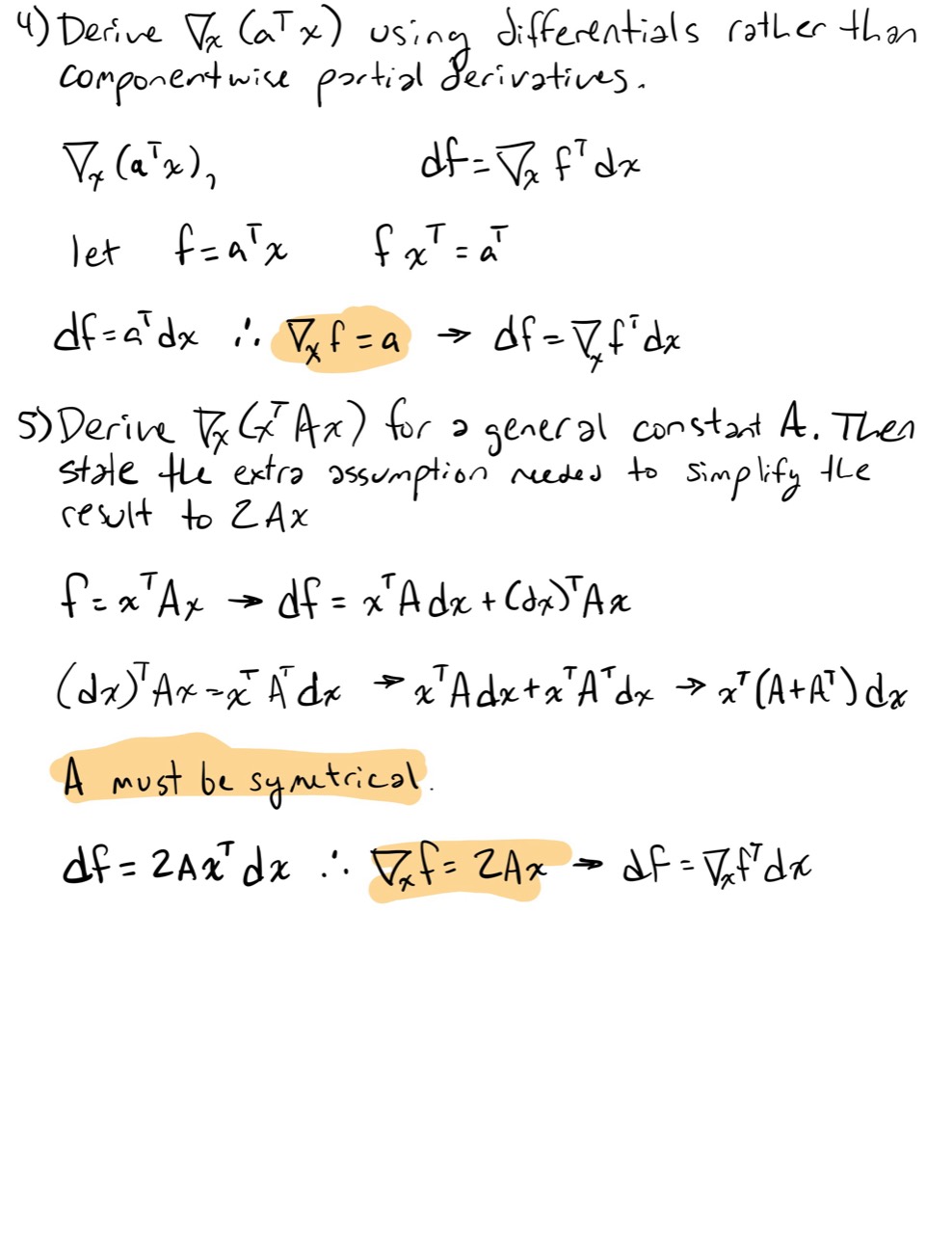
Derive $\nabla_x(a^Tx)$ using differentials rather than componentwise partial derivatives.
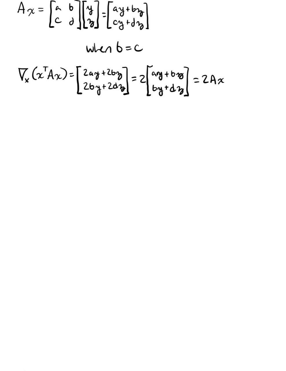
Derive $\nabla_x(x^TAx)$ for a general constant $A$ . Then state the extra assumption needed to simplify the result to $2Ax$ .
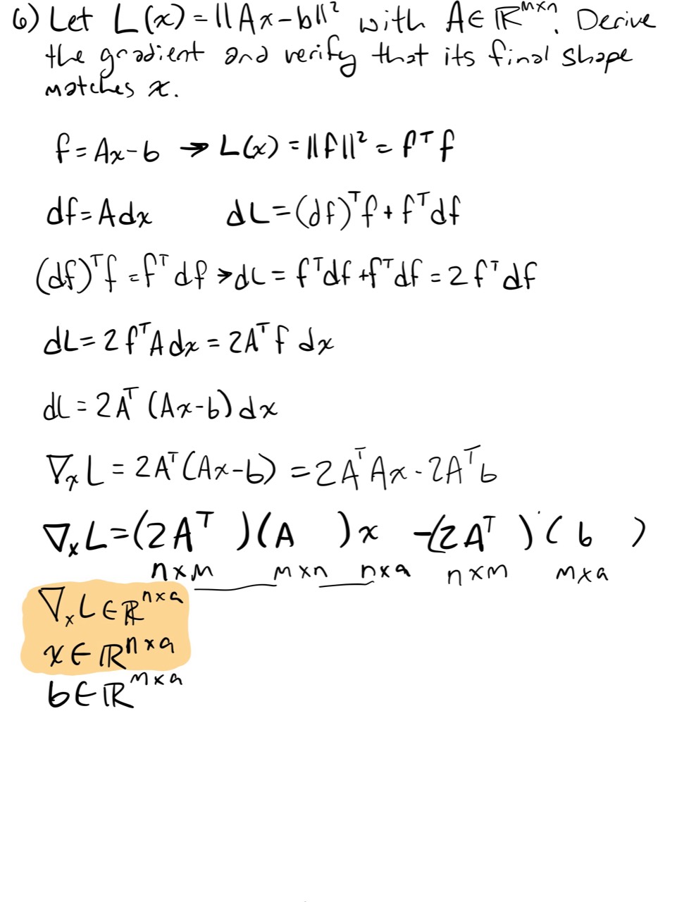
Let $L(x)=\lVert Ax-b\rVert^2$ with $A\in\mathbb R^{m\times n}$ . Derive the gradient and verify that its final shape matches $x$ .
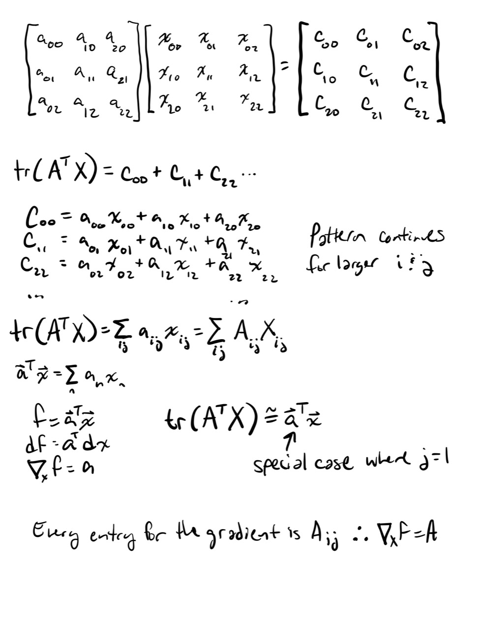
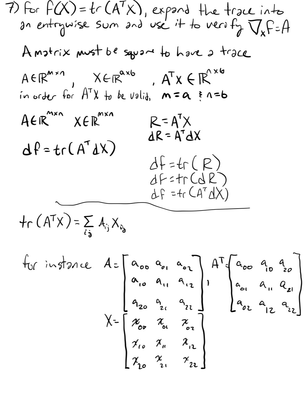
For $f(X)=\operatorname{tr}(A^TX)$ , expand the trace into an entrywise sum and use it to verify $\nabla_Xf=A$ .
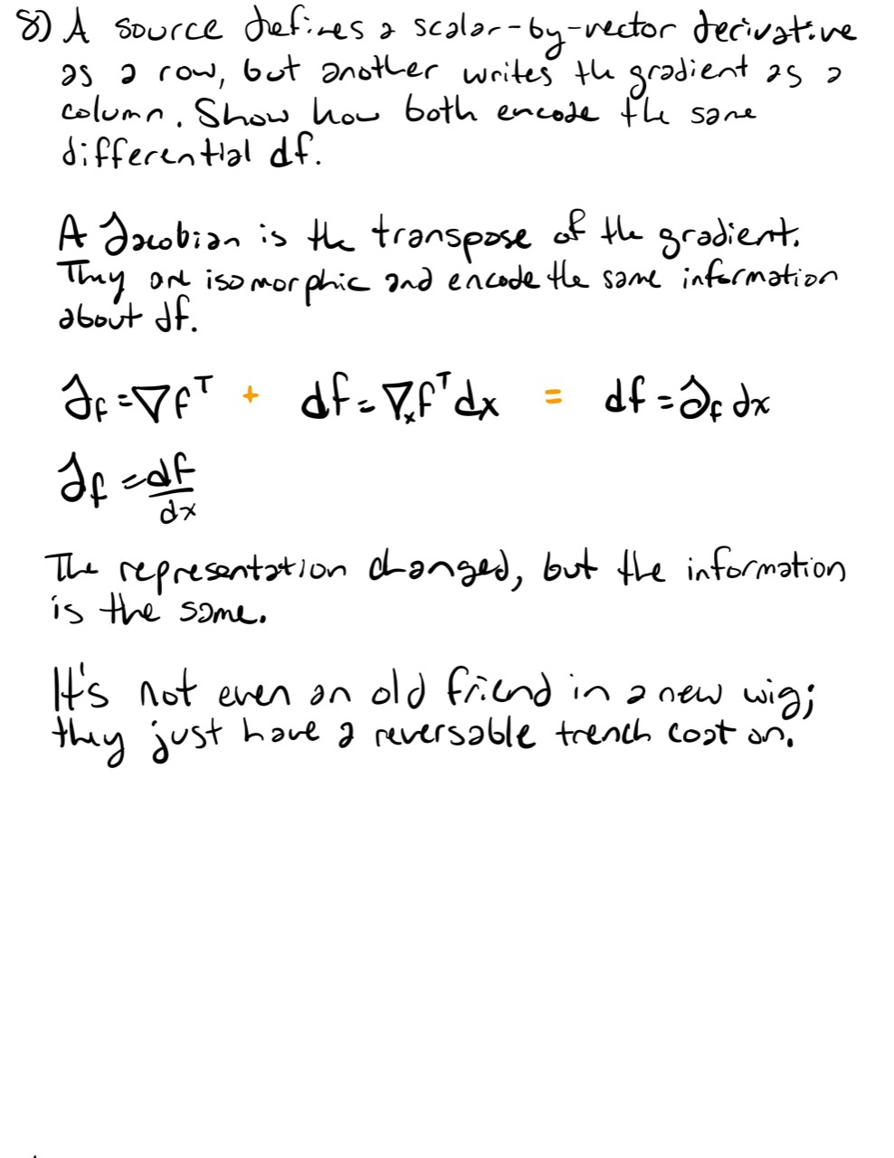
A source defines a scalar-by-vector derivative as a row but another writes the gradient as a column. Show how both encode the same differential $df$ .
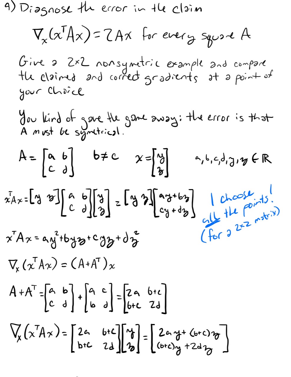
Diagnose the error in the claim $\nabla_x(x^TAx)=2Ax$ for every square $A$ . Give a $2\times2$ nonsymmetric example and compare the claimed and correct gradients at a point of your choice.
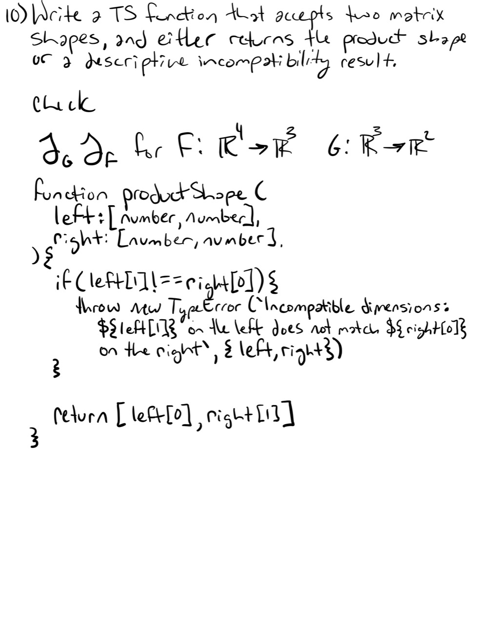
Write a TypeScript function that accepts two matrix shapes and either returns the product shape or a descriptive incompatibility result. Use it to type-check $J_GJ_F$ for $F:\mathbb R^4\to\mathbb R^3$ and $G:\mathbb R^3\to\mathbb R^2$ .

Summary

A derivative is a local linear map; its array shape is a representation of that map.
This course uses output-by-input Jacobians and column gradients for scalar outputs.
Numerator and denominator layouts transpose the same table of partial derivatives.
$dF=J_Fdx$ describes forward displacement propagation.
$\nabla_xL=J_F^T\nabla_FL$ describes reverse column-gradient propagation.
Differentials expose gradients by matching $df=(\nabla_xf)^Tdx$ .
Matrix gradients use $df=\operatorname{tr}((\nabla_Xf)^TdX)$ .
Shape checking catches many transpose and composition errors, but it does not replace differentiating the actual operation.

Next Lesson

Lesson 39 develops Taylor series and local approximation. It will connect the gradient to the best first-order model and the Hessian to the second-order correction.

Completed Exercises

Handwritten work submitted after completing this lesson.