Lesson 39: Taylor Series and Local Approximation

Goal

Turn derivatives into local predictive models.

The central idea is:

Near an anchor point, a smooth function behaves like a low-degree polynomial whose coefficients are determined by derivatives at that anchor.

A gradient is not merely a direction used by an optimizer. It is the coefficient of the best first-order local model. A Hessian is not merely a curvature table. It supplies the second-order correction that lets the local model bend.

Why Local Models Matter

Suppose evaluating a function is expensive or its formula is complicated. If we already know the function and its derivatives at a point $a$ , then we can ask a smaller question:

What simple function behaves like the original function for points close to $a$ ?

The answer begins with a constant, then adds increasingly detailed corrections:

known height
+ local slope correction
+ local curvature correction
+ higher-order corrections

This is compression. Instead of carrying the whole function, we carry a local polynomial model.

The model is trustworthy only locally. Moving far from the anchor can make omitted higher-order behavior dominate.

Notation / Symbol Table

Symbol	Plain-English name	Meaning
$f$	target function	The function being approximated.
$a$	anchor point	The point where values and derivatives are known.
$x$	target point	The nearby point where we want a prediction.
$h=x-a$	displacement	How far and in which direction we move from the anchor.
$T_0(x;a)$	zero-order model	The constant prediction $f(a)$ .
$T_1(x;a)$	first-order model	Constant plus slope or gradient correction.
$T_2(x;a)$	second-order model	First-order model plus curvature correction.
$R_k(x;a)$	remainder	The approximation error $f(x)-T_k(x;a)$ .
$H_f(a)$	Hessian at $a$	Matrix describing how the gradient changes near $a$ .

The semicolon in $T_k(x;a)$ separates the point being predicted from the fixed anchor used to build the model.

Start With One Variable

For a smooth scalar function $f:\mathbb R\to\mathbb R$ , write the target point as:

x=a+h.

The displacement $h$ is the small quantity. The Taylor polynomial through second order is:

f(a+h) \approx f(a)+f'(a)h+\frac{1}{2}f''(a)h^2.

Equivalently:

T_2(x;a) = f(a)+f'(a)(x-a)+\frac{1}{2}f''(a)(x-a)^2.

Each term has a distinct job:

Term	Information supplied	Geometric job
$f(a)$	function value	Places the model at the correct height.
$f'(a)h$	first derivative	Tilts the model with the correct local slope.
$\frac12 f''(a)h^2$	second derivative	Bends the model with the correct local curvature.

Why The Factorial Appears

The quadratic correction contains $1/2=1/2!$ because differentiating $h^2$ twice produces a factor of $2$ :

\frac{d^2}{dh^2}\left(c_2h^2\right)=2c_2.

To make that second derivative equal $f''(a)$ , choose:

c_2=\frac{f''(a)}{2!}.

The same matching rule gives the degree- $k$ Taylor polynomial:

T_k(x;a) = \sum_{j=0}^{k} \frac{f^{(j)}(a)}{j!}(x-a)^j.

The factorial cancels the repeated factors created when a power is differentiated back down.

Worked Example: Approximating The Exponential

Let:

f(x)=e^x

and anchor at $a=0$ . Every derivative of $e^x$ is $e^x$ , so at zero:

f(0)=f'(0)=f''(0)=1.

The approximations are:

T_0(x;0)=1,

T_1(x;0)=1+x,

T_2(x;0)=1+x+\frac{x^2}{2}.

At $x=0.1$ :

T_1(0.1;0)=1.1,

T_2(0.1;0)=1.105,

while:

e^{0.1}\approx1.105170.

The curvature term repairs most of the first-order error because the displacement is small.

The Remainder Is The Missing Behavior

Define the remainder after a degree- $k$ approximation by:

R_k(x;a)=f(x)-T_k(x;a).

For a sufficiently smooth function near $a$ , the local scaling is:

R_0=O(|h|), \qquad R_1=O(|h|^2), \qquad R_2=O(|h|^3).

Read $O(|h|^p)$ here as a scaling statement: close enough to the anchor, the error is bounded by a constant times $|h|^p$ .

This gives a useful experiment. If $h$ is halved, then locally:

Model	Leading error scale	Expected error factor after halving $h$
Constant	$\lvert h\rvert$	about $1/2$
First order	$\lvert h\rvert^2$	about $1/4$
Second order	$\lvert h\rvert^3$	about $1/8$

These ratios are asymptotic, not exact promises at arbitrary distances.

Multivariable First-Order Approximation

Now let:

f:\mathbb R^n\to\mathbb R, \qquad x=a+h.

The first-order Taylor model is:

T_1(a+h;a) = f(a)+\nabla f(a)^T h.

The shape check is:

\underbrace{T_1}_{1\times1} = \underbrace{f(a)}_{1\times1} + \underbrace{\nabla f(a)^T}_{1\times n} \underbrace{h}_{n\times1}.

This is the differential from Lesson 38 with a finite but small displacement:

df=\nabla f(a)^Tdx \quad\longrightarrow\quad f(a+h)-f(a)\approx\nabla f(a)^Th.

The approximation is a tangent hyperplane. The gradient supplies its coefficients.

Multivariable Second-Order Approximation

The Hessian supplies the curvature correction:

T_2(a+h;a) = f(a) +\nabla f(a)^Th +\frac12h^TH_f(a)h.

The quadratic form is scalar:

\underbrace{h^T}_{1\times n} \underbrace{H_f(a)}_{n\times n} \underbrace{h}_{n\times1} \in\mathbb R.

The term $h^TH_f(a)h$ measures curvature along the actual displacement $h$ . If $h$ is not a unit vector, its length contributes twice because $h$ appears on both sides of the Hessian.

Worked Example: A Quadratic Function

Let:

f(x,y)=x^2+xy+2y^2.

Anchor at:

a= \begin{bmatrix} 1\\-1 \end{bmatrix},

and use displacement:

h= \begin{bmatrix} 0.2\\0.1 \end{bmatrix}.

First compute the local data:

f(a)=2,

\nabla f(x,y)= \begin{bmatrix} 2x+y\\x+4y \end{bmatrix}, \qquad \nabla f(a)= \begin{bmatrix} 1\\-3 \end{bmatrix},

H_f= \begin{bmatrix} 2&1\\1&4 \end{bmatrix}.

The first-order model predicts:

T_1=2+ \begin{bmatrix} 1&-3 \end{bmatrix} \begin{bmatrix} 0.2\\0.1 \end{bmatrix} =1.9.

The second-order correction is:

\frac12h^TH_fh=0.08.

Therefore:

T_2=1.98.

The target point is $(1.2,-0.9)$ , and direct evaluation also gives:

f(1.2,-0.9)=1.98.

The second-order model is exact because the original function is quadratic. There are no third- or higher-order terms to omit.

A Local Model Is Not A Global Identity

The approximation symbol matters:

f(a+h)\approx T_k(a+h;a).

Equality holds only in special cases, such as using a second-order model for a quadratic function. For a general function, accuracy depends on:

distance from the anchor,
size of omitted derivatives,
smoothness near the path from $a$ to $a+h$ ,
and the chosen approximation order.

A high-order polynomial can still be poor far from its anchor. More terms increase local fidelity; they do not make locality disappear.

From Taylor Models To Optimization

Let $L(\theta)$ be a loss near current parameters $\theta$ . For a proposed update $s$ , the first-order model is:

L(\theta+s) \approx L(\theta)+\nabla L(\theta)^Ts.

Choosing:

s=-\eta\nabla L(\theta)

gives the predicted change:

\nabla L(\theta)^Ts = -\eta\lVert\nabla L(\theta)\rVert^2,

which is negative whenever the gradient is nonzero. This is the local-model justification for gradient descent.

The second-order model is:

L(\theta+s) \approx L(\theta) +\nabla L(\theta)^Ts +\frac12s^TH_L(\theta)s.

If the Hessian is invertible and the quadratic model is locally appropriate, setting the model’s gradient with respect to $s$ to zero gives:

s_{\text{Newton}} = -H_L(\theta)^{-1}\nabla L(\theta).

Gradient descent trusts slope and controls distance with a learning rate. Newton’s method also uses curvature to rescale and rotate the proposed step.

Why This Matters For Neural Networks

Neural-network training repeatedly builds implicit local models of a loss landscape:

Backpropagation supplies the gradient for a first-order model.
Learning rates limit how far we trust that local model.
Hessian information describes curvature but is expensive to store and use at modern model scale.
Curvature approximations and Hessian-vector products try to capture useful second-order structure without materializing the full Hessian.
Flat and sharp directions matter because one scalar learning rate acts across many directions with different curvature.

The Taylor viewpoint unifies these facts: optimization methods differ partly in what local model they build and how much of it they can afford to use.

Connection To Programming

A local quadratic model can be represented without hiding its assumptions:

type Vector = readonly number[];
type Matrix = readonly (readonly number[])[];

const dot = (left: Vector, right: Vector): number =>
  left.reduce((sum, value, index) => sum + value * right[index]!, 0);

const multiplyMatrixVector = (
  matrix: Matrix,
  vector: Vector,
): Vector => matrix.map((row) => dot(row, vector));

const secondOrderTaylor = ({
  valueAtAnchor,
  gradientAtAnchor,
  hessianAtAnchor,
  displacement,
}: Readonly<{
  valueAtAnchor: number;
  gradientAtAnchor: Vector;
  hessianAtAnchor: Matrix;
  displacement: Vector;
}>): number => {
  const linearCorrection = dot(gradientAtAnchor, displacement);
  const curvatureAlongDisplacement = dot(
    displacement,
    multiplyMatrixVector(hessianAtAnchor, displacement),
  );

  return valueAtAnchor + linearCorrection + 0.5 * curvatureAlongDisplacement;
};

The names preserve the mathematical roles. The function receives local information and a displacement; it does not pretend to know the original function globally.

Common Mistakes

Evaluating Derivatives At The Target Instead Of The Anchor

A Taylor model is built from $f(a)$ , $f'(a)$ , and higher derivatives at the fixed anchor $a$ . Evaluating each coefficient at $x$ changes the construction.

Forgetting The Displacement

The linear term is not merely $f'(a)$ or $\nabla f(a)$ . It is the derivative applied to $h=x-a$ .

Dropping The One-Half

The second-order term is $\frac12f''(a)h^2$ in one variable and $\frac12h^TH_f(a)h$ in several variables.

Treating The Hessian Term As A Matrix Output

For a scalar function, $h^THh$ is a scalar quadratic form. Shape checking should reduce the full expression to $1\times1$ .

Assuming More Terms Guarantee Global Accuracy

Taylor models organize local derivative information. Their useful region depends on the function and anchor, not just the polynomial degree.

Confusing Approximation Error With Numerical Rounding

Remainder error comes from omitted mathematical terms. Floating-point error comes from numerical representation and computation. They are different sources of error.

Exercises

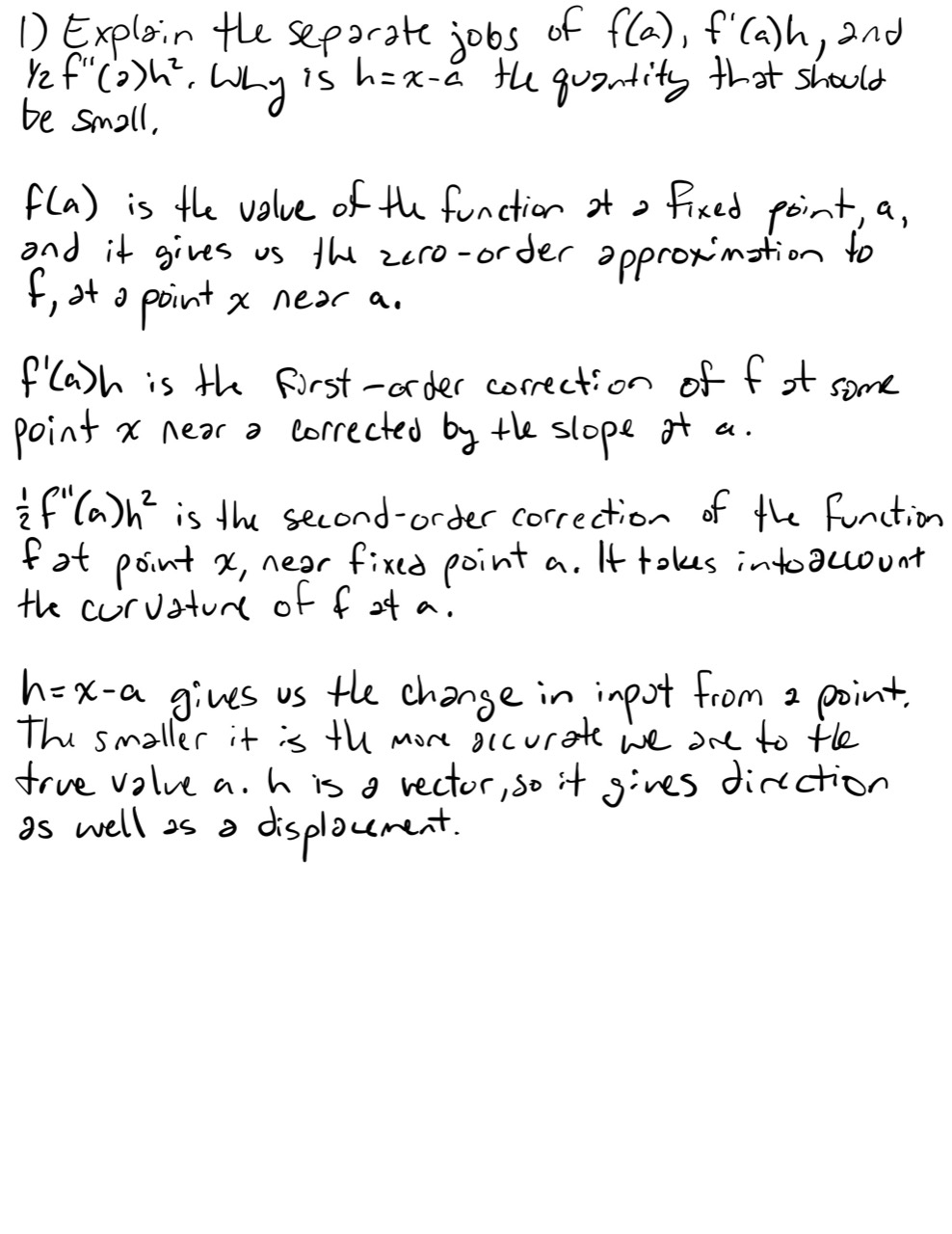
In plain language, explain the separate jobs of $f(a)$ , $f'(a)h$ , and $\frac12f''(a)h^2$ . Why is $h=x-a$ the quantity that should be small?
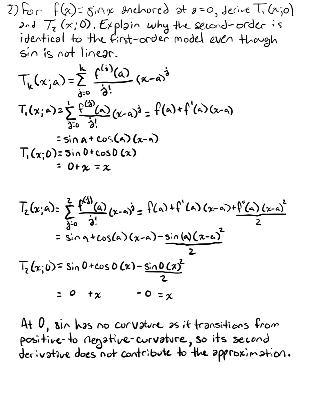
For $f(x)=\sin x$ anchored at $a=0$ , derive $T_1(x;0)$ and $T_2(x;0)$ . Explain why the second-order model is identical to the first-order model even though $\sin x$ is not linear.
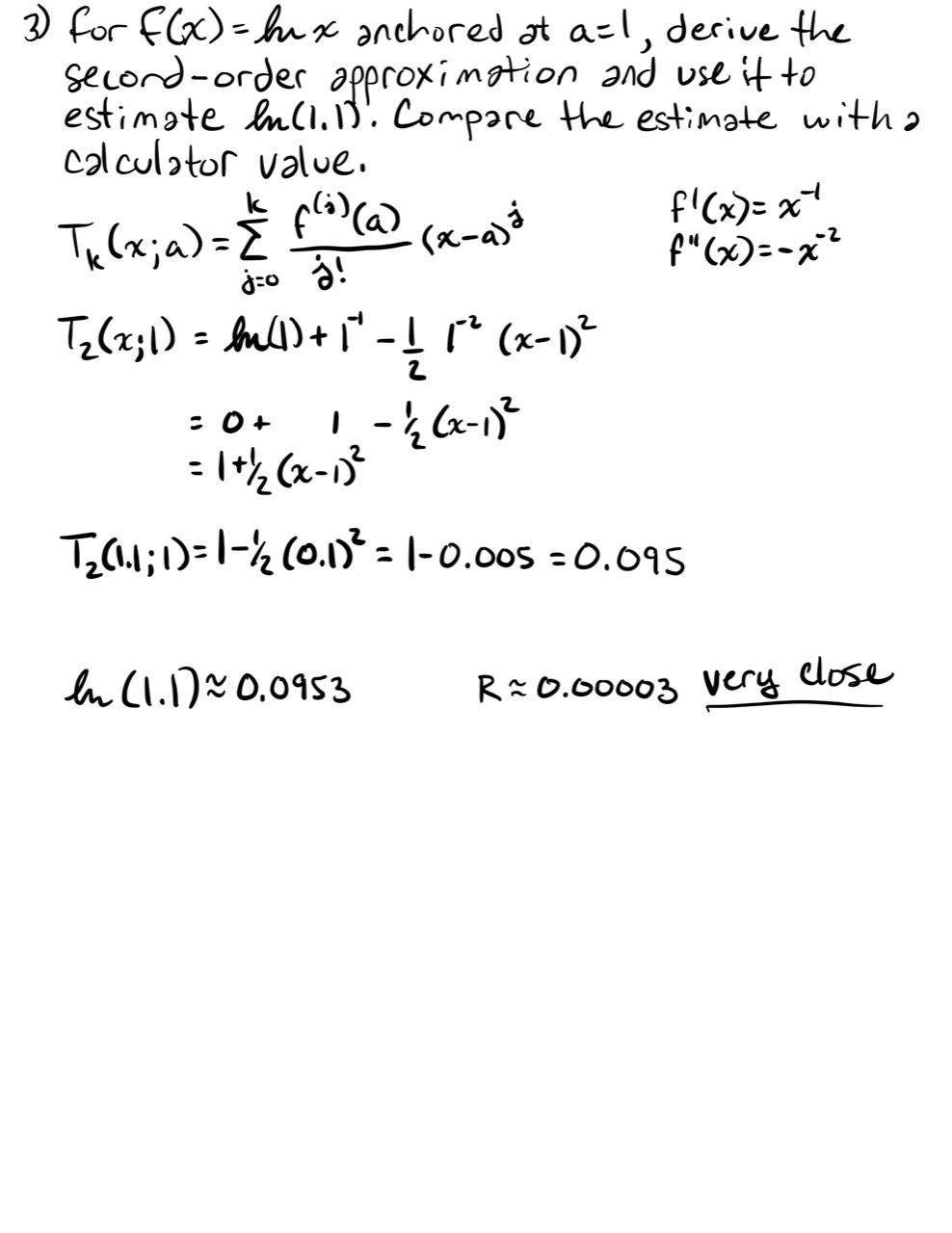
For $f(x)=\ln x$ anchored at $a=1$ , derive the second-order approximation and use it to estimate $\ln(1.1)$ . Compare the estimate with a calculator value.
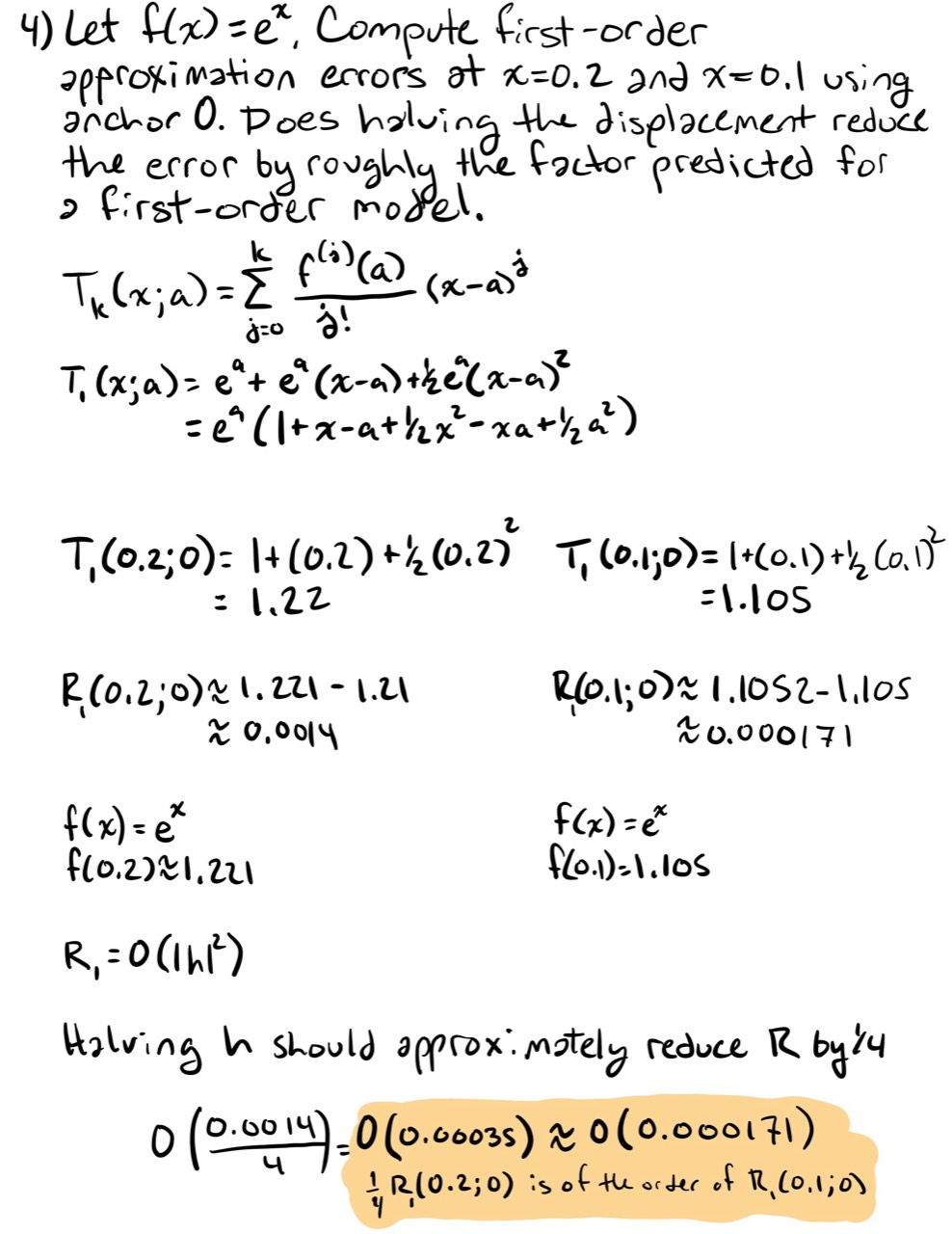
Let $f(x)=e^x$ . Compute first-order approximation errors at $x=0.2$ and $x=0.1$ using anchor $0$ . Does halving the displacement reduce the error by roughly the factor predicted for a first-order model?
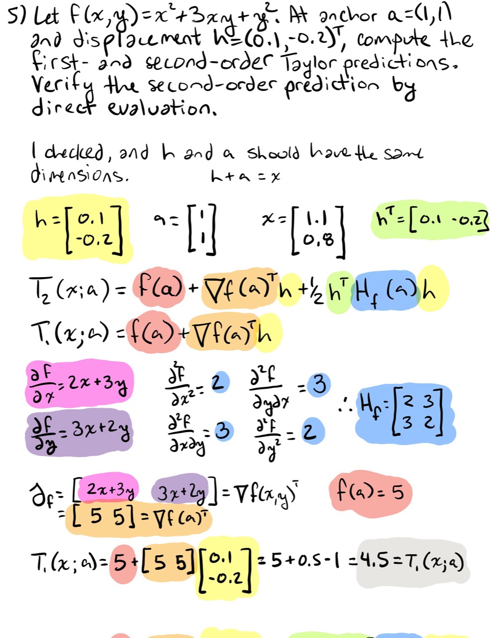
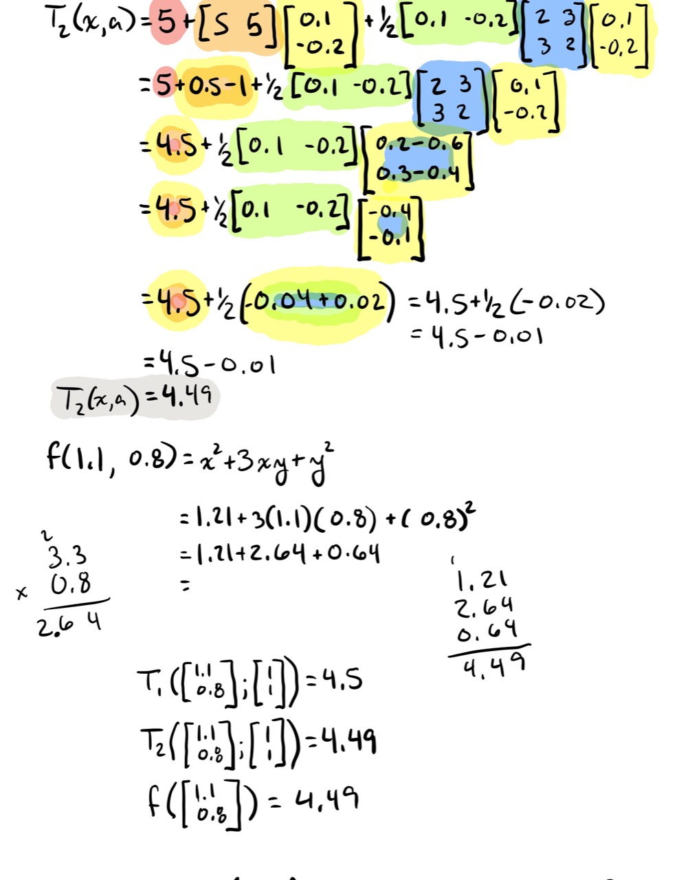
Let $f(x,y)=x^2+3xy+y^2$ . At anchor $a=(1,1)$ and displacement $h=(0.1,-0.2)^T$ , compute the first- and second-order Taylor predictions. Verify the second-order prediction by direct evaluation.
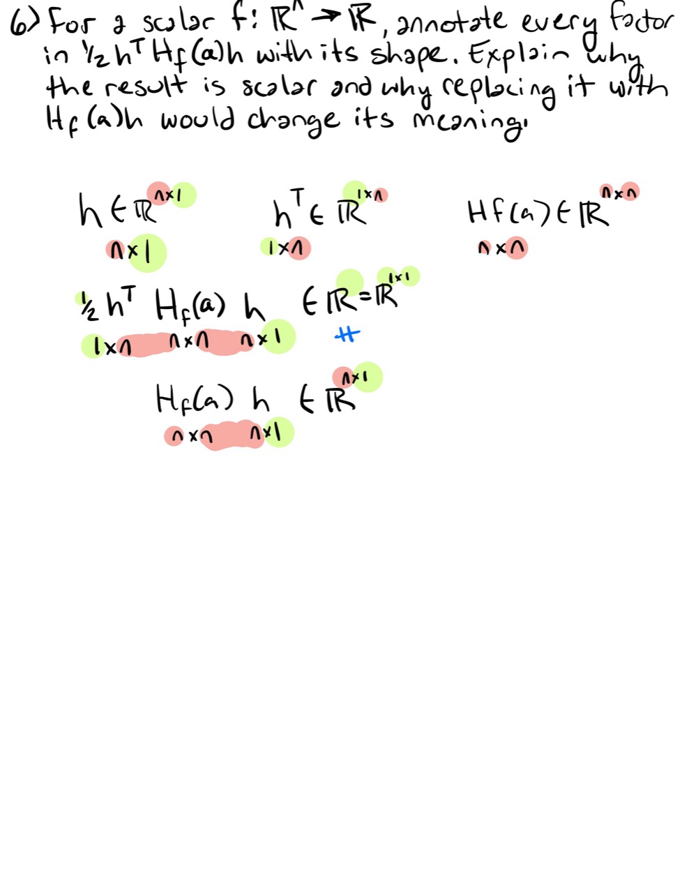
For a scalar $f:\mathbb R^n\to\mathbb R$ , annotate every factor in $\frac12h^TH_f(a)h$ with its shape. Explain why the result is scalar and why replacing it with $H_f(a)h$ would change its meaning.
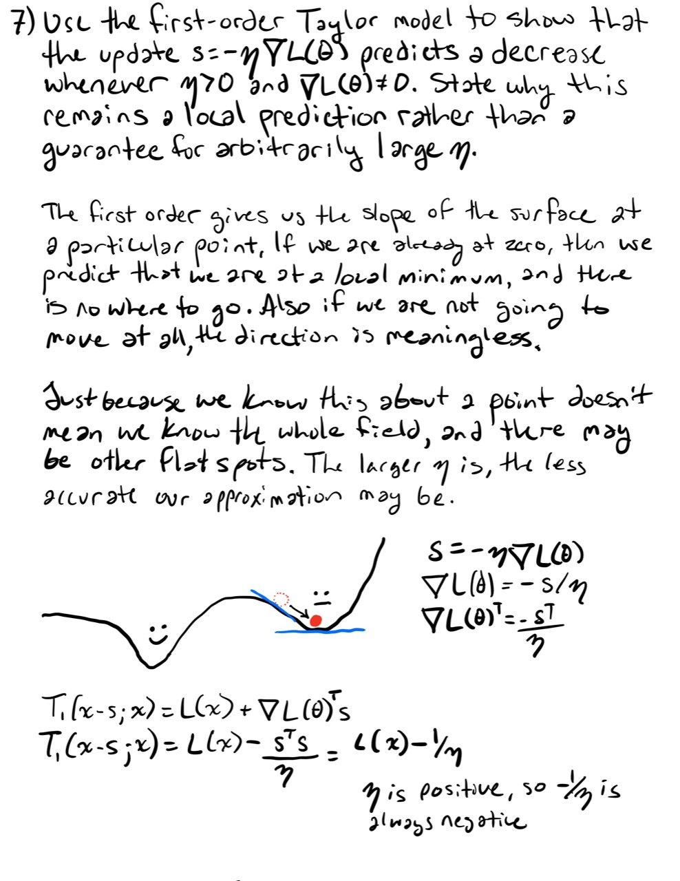
Use the first-order Taylor model to show that the update $s=-\eta\nabla L(\theta)$ predicts a decrease whenever $\eta>0$ and $\nabla L(\theta)\ne0$ . State why this remains a local prediction rather than a guarantee for arbitrarily large $\eta$ .
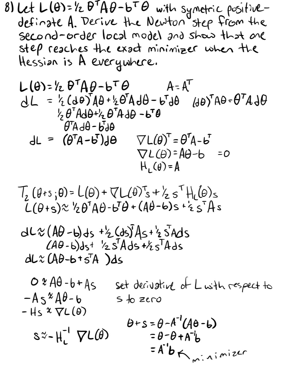
Let $L(\theta)=\frac12\theta^TA\theta-b^T\theta$ with symmetric positive-definite $A$ . Derive the Newton step from the second-order local model and show that one step reaches the exact minimizer when the Hessian is $A$ everywhere.
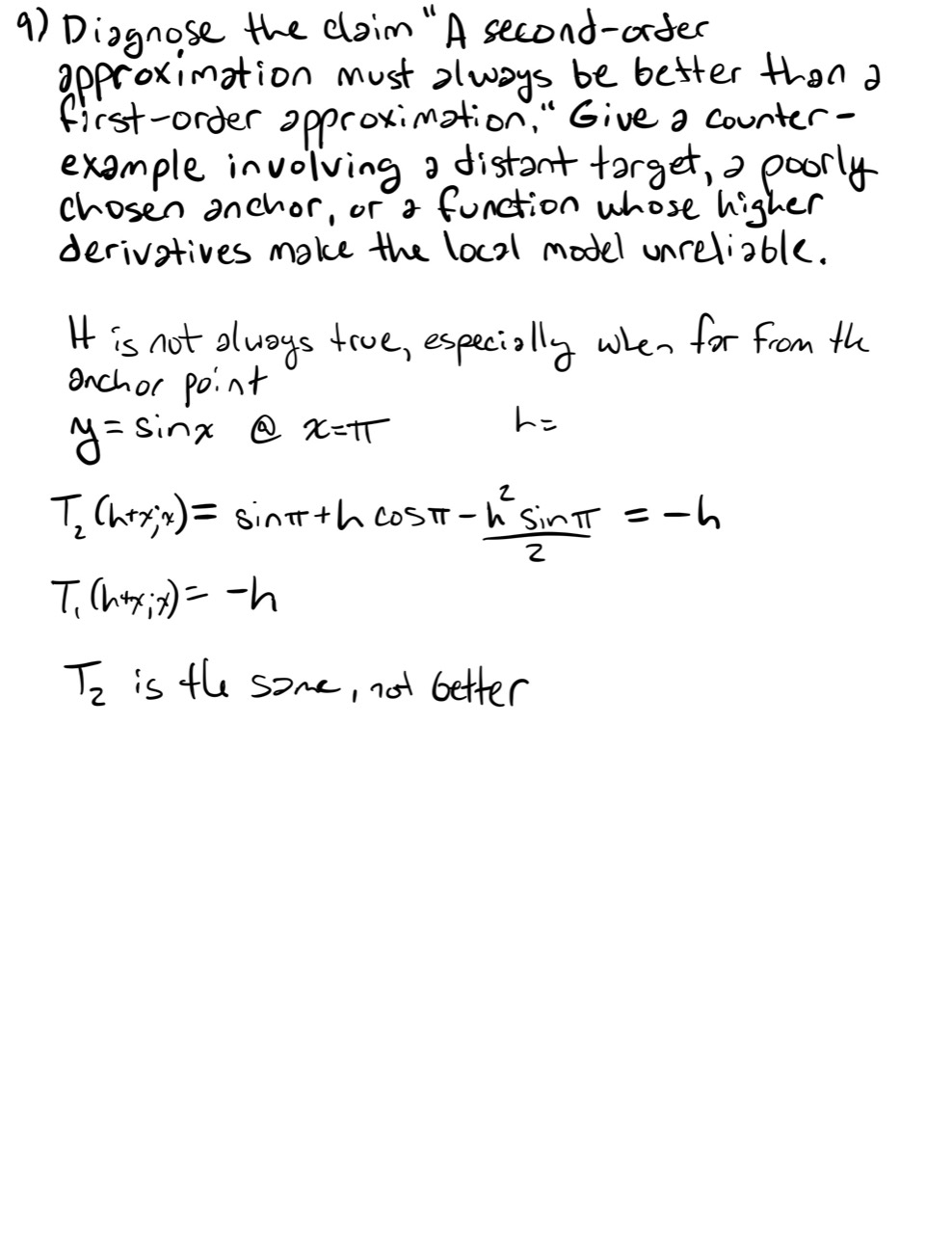
Diagnose the claim: “A second-order approximation must always be better than a first-order approximation.” Give a counterexample involving a distant target, a poorly chosen anchor, or a function whose higher derivatives make the local model unreliable.
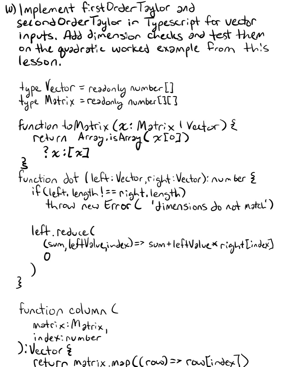
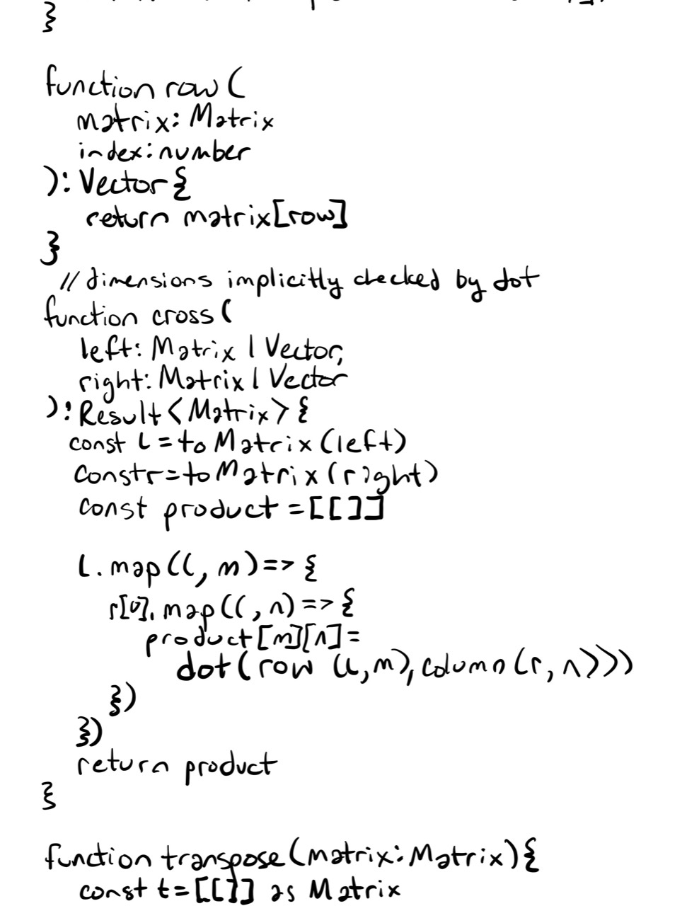
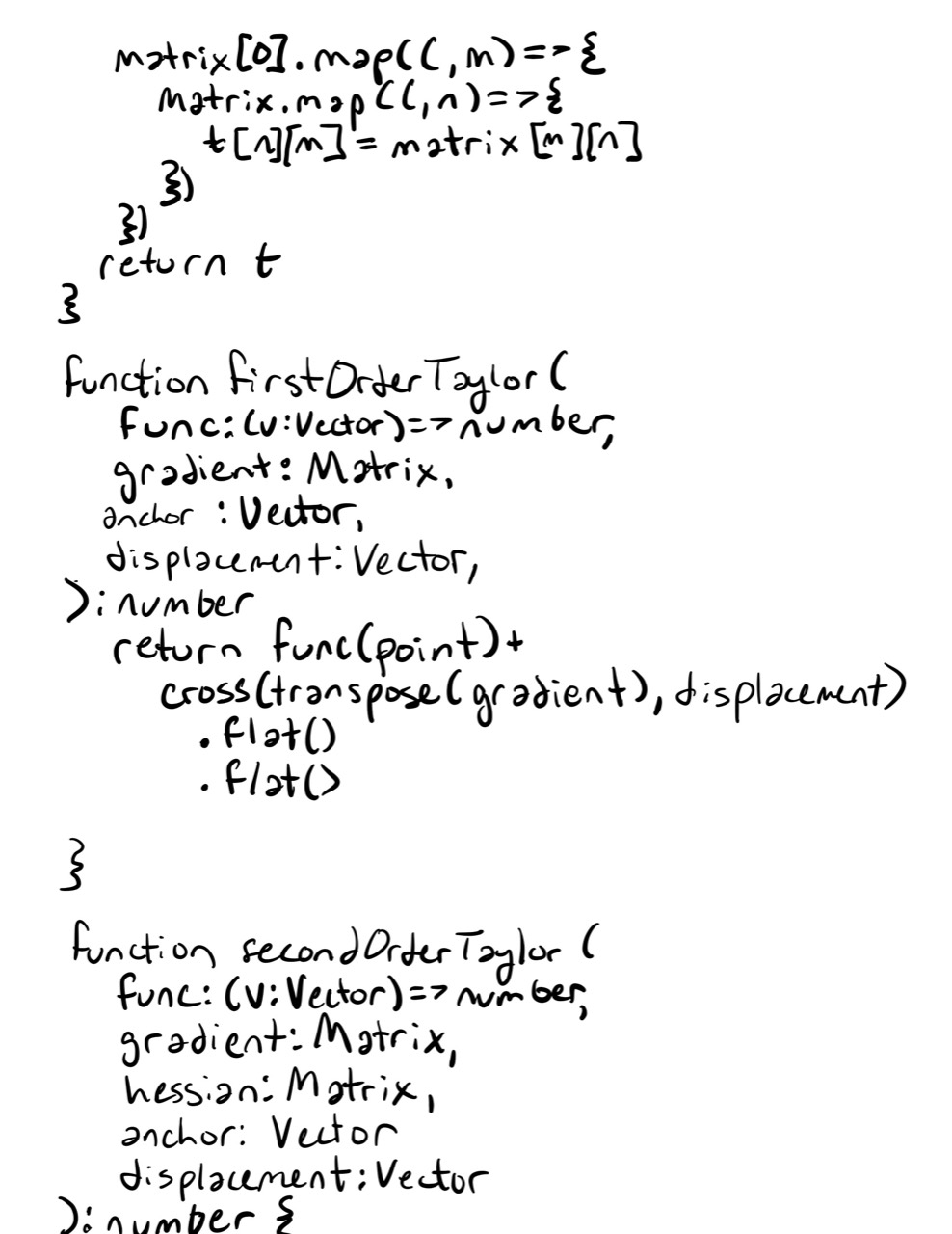
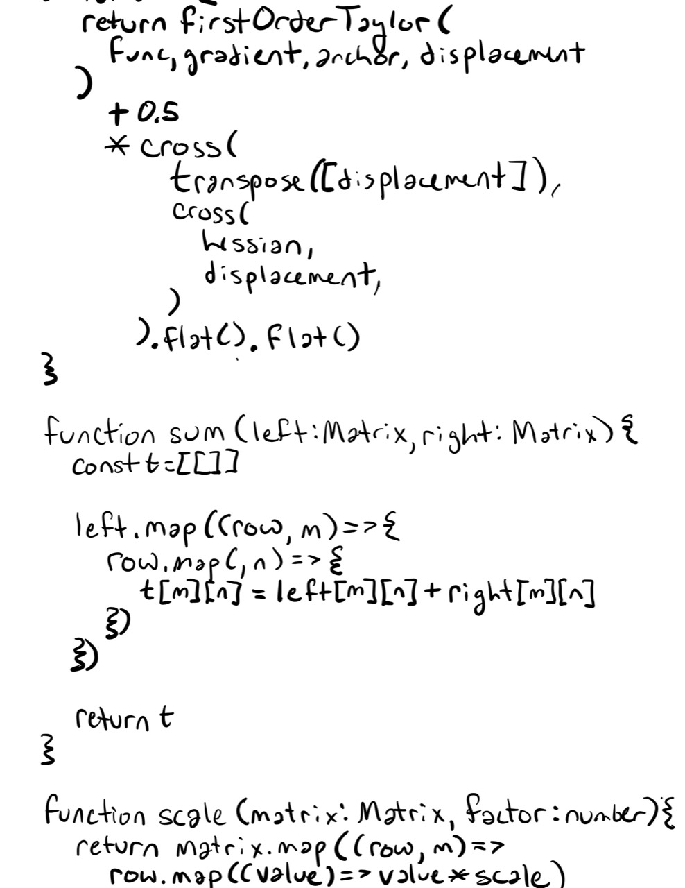
Implement firstOrderTaylor and secondOrderTaylor in TypeScript for vector inputs. Add dimension checks and test them on the quadratic worked example from this lesson.

Readiness Check

You are ready to move into neural-network layers when you can:

identify the anchor and displacement before calculating,
reconstruct first- and second-order models rather than recall them as unexplained formulas,
use gradient and Hessian shapes correctly,
predict how local error changes when the displacement shrinks,
and explain gradient descent as optimization of a local first-order model.

Summary

Taylor approximation replaces a complicated function locally with a derivative-matched polynomial.
The function value sets height, the gradient sets slope, and the Hessian supplies curvature.
First-order error is locally quadratic in displacement; second-order error is locally cubic under suitable smoothness.
In several variables, the linear correction is $\nabla f(a)^Th$ and the quadratic correction is $\frac12h^TH_f(a)h$ .
A quadratic function is represented exactly by its second-order Taylor model.
Gradient descent and Newton’s method can be understood as decisions made from first- and second-order local models.
Local accuracy does not imply global accuracy.

Next Lesson

Lesson 40 begins the neural-network phase with perceptrons and linear layers. It will turn affine maps into trainable units, connect weights and biases to decision boundaries, and reuse the local derivative machinery developed in Lessons 35–39.