Goal
Turn the affine maps you already know into trainable units.
A perceptron or linear layer does not introduce new linear algebra. It assigns machine-learning roles to familiar objects:
input vector
→ weighted sum
→ bias shift
→ optional activation
→ output
The core computation is an affine map:
A neural network is built by composing many such maps with nonlinear functions between them.
Why Start Here
Suppose an input has two features:
We want a model that produces a score saying which side of a boundary the point lies on. Choose weights:
and a bias . The score is:
The model may classify using the sign:
The boundary itself is where the model is undecided:
That equation defines a line in two dimensions, a plane in three dimensions, and a hyperplane in higher dimensions.
Notation / Symbol Table
| Symbol | Plain-English name | Meaning |
|---|---|---|
| input vector | The features supplied to one unit. | |
| weight vector | Coefficients controlling how each input feature affects the score. | |
| bias | A scalar offset that moves the boundary without rotating it. | |
| pre-activation | The affine score before applying a nonlinear function. | |
| activation function | A scalar function applied to the pre-activation. | |
| activation | The unit’s output after the activation function. | |
| weight matrix | Stacks output-unit weight vectors as rows. | |
| bias vector | One bias for each of the output units. | |
| layer pre-activation | The vector of all unit scores in a linear layer. |
A Perceptron Is An Affine Map Plus A Decision Rule
The word linear is used loosely in neural-network programming. The map:
is technically affine because it includes the constant term . It is linear only when .
The distinction matters geometrically:
- must pass through the origin.
- may be shifted away from the origin.
The original perceptron used a hard threshold. Modern neural networks more often use differentiable or piecewise-differentiable activations, but the affine core is the same.
The Weight Vector Is Normal To The Boundary
Consider the decision boundary:
Let and be any two points on that boundary. Then:
and:
Subtract the equations:
So every displacement lying along the boundary is orthogonal to . Therefore points straight across the boundary.
This gives the weights two simultaneous interpretations:
- As coefficients in a weighted sum.
- As the normal direction of the decision boundary.
The score changes most rapidly when moving parallel to .
What The Bias Does
Holding fixed preserves the boundary’s orientation. Changing translates the boundary.
For a one-dimensional input:
has boundary location:
provided .
In higher dimensions, the signed score scaled by the weight norm gives signed distance from the boundary:
The sign tells which side of the boundary contains . The magnitude tells how far away it is in the normal direction.
Worked Example: A Two-Feature Perceptron
Let:
For input:
compute:
A hard threshold would classify this point as positive because .
The boundary is:
or:
The vector is perpendicular to this line.
From One Unit To A Linear Layer
A single unit produces one scalar. A layer with units produces scores.
Let each unit have its own weight vector . Stack their transposes as rows:
Stack the biases into:
Then every unit can be evaluated at once:
The shape check is:
Each row of asks a different linear question about the same input.
Worked Example: A Three-Output Layer
Let:
Then:
Adding the bias gives:
The layer has transformed a two-dimensional input into a three-dimensional representation.
Why Activations Are Needed
Composing affine maps without nonlinear activations does not create a more expressive class of functions.
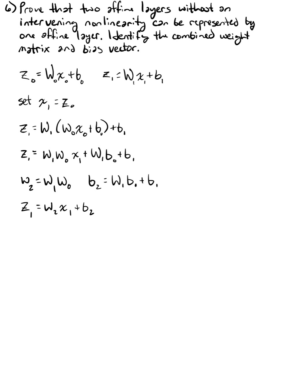
Suppose:
and:
Substitute the first into the second:
The composition is still one affine map.
A nonlinear activation prevents this collapse:
The nonlinearity is what lets depth create genuinely new functions.
Common Activation Examples
Hard Threshold
Useful for understanding the historical perceptron, but unsuitable for ordinary gradient-based training because its derivative is zero almost everywhere and undefined at zero.
Sigmoid
Maps scores into . It is useful for probabilities and binary outputs, though deep networks often avoid it in hidden layers because large positive or negative inputs produce small gradients.
ReLU
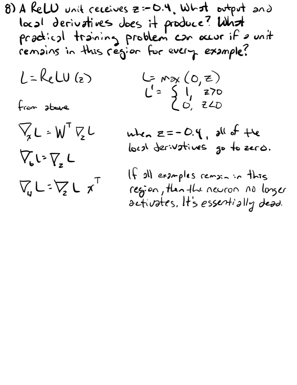
Piecewise linear and inexpensive. Its derivative is:
At , software chooses a convention, commonly zero.
The Local Derivatives Of A Single Unit
Let:
Treat , , and as separate inputs to this computation.
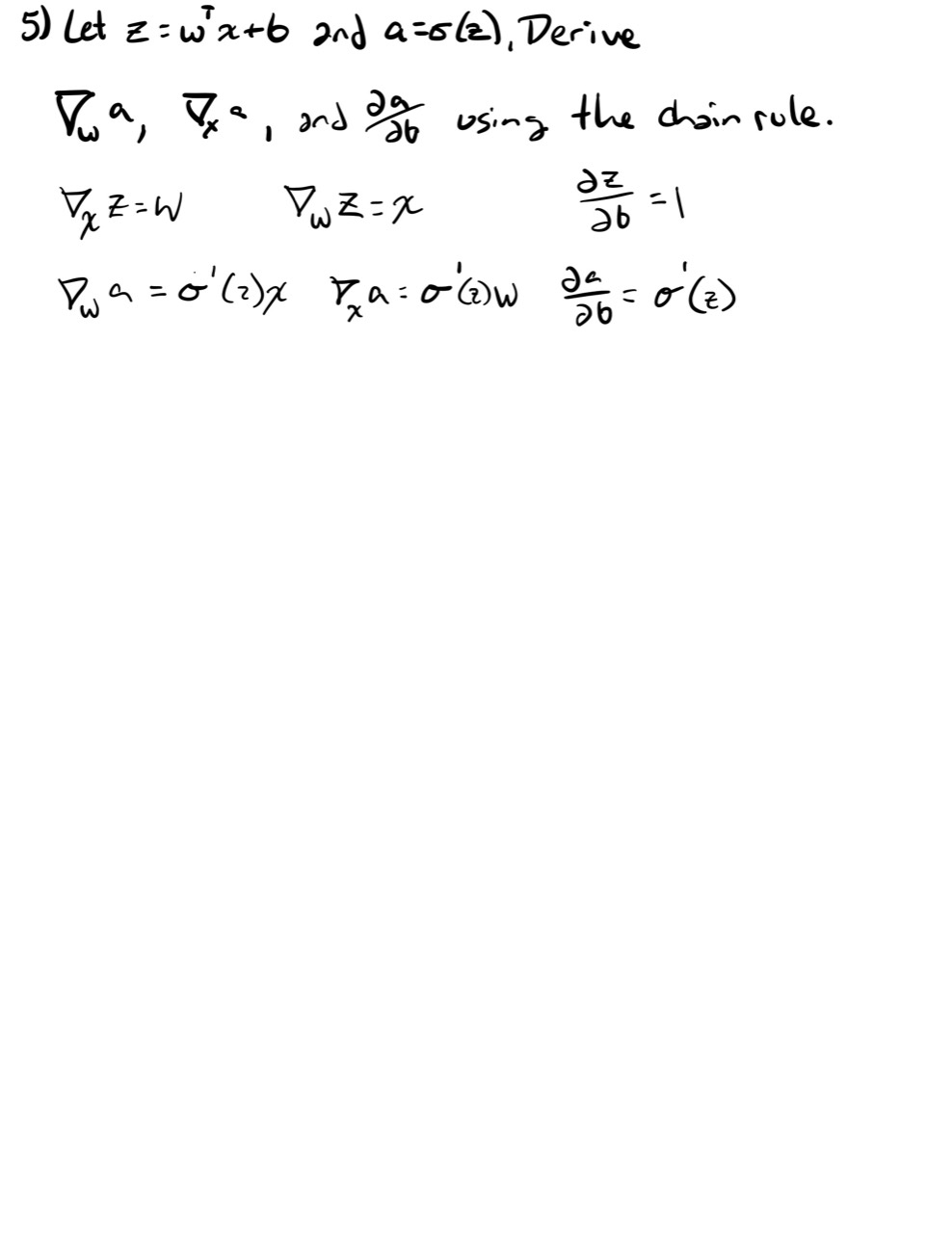
The derivative with respect to the input is:
The derivative with respect to the weights is:
The derivative with respect to the bias is:
These formulas are symmetric for a reason. The scalar score is the dot product pairing between and . Holding either side fixed makes the other side’s gradient equal to the fixed vector.
For:
the chain rule gives:
and:
The forward pass stores , , , and . The backward pass multiplies the incoming sensitivity by these local derivatives.
Gradients For A Linear Layer
For:
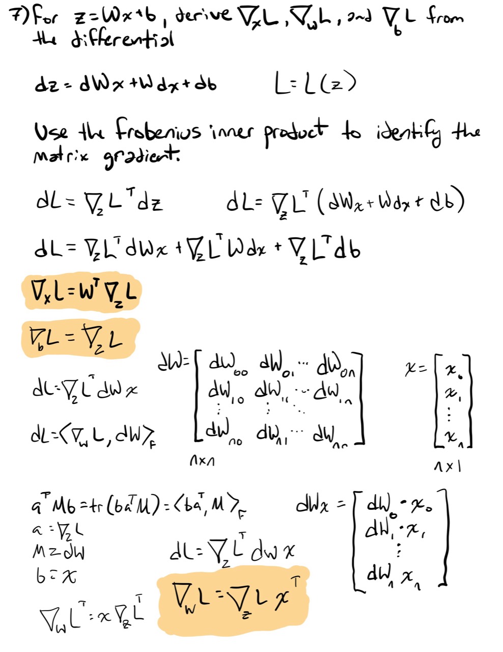
suppose a scalar loss produces an incoming sensitivity:
Then:
and:
Check the shapes:
and:
The weight gradient is an outer product. Each output sensitivity scales the input vector to produce one row of the matrix gradient.
A Useful Programming View
A linear layer can keep forward data and backward behavior together:
type Vector = readonly number[];
type Matrix = readonly (readonly number[])[];

type LinearCache = Readonly<{
  input: Vector;
}>;

type LinearLayer = Readonly<{
  weights: Matrix;
  bias: Vector;
}>;

type LinearBackward = Readonly<{
  inputGradient: Vector;
  weightGradient: Matrix;
  biasGradient: Vector;
}>;
The layer’s forward pass computes and stores the input. Its backward pass receives , then computes the three gradients above.
This is the first reusable trainable operation in the neural-network implementation path.
Connection To Category Theory
The useful connection is composition, not terminology.
A linear layer is a morphism-like computational component with a typed input and output:
R^n → R^mLayers compose only when adjacent shapes match. The forward maps compose in the ordinary direction. Reverse-mode sensitivities travel backward through the transposed local linear maps.
The nonlinear activation is crucial because a category containing only affine maps remains closed under composition: composing more arrows does not escape the same family of functions.
Why This Matters For Machine Learning
Linear layers appear throughout modern models:
- Feature classifiers use .
- Multiclass classifiers use one row of per class.
- Hidden neural-network layers learn new feature coordinates.
- Convolution can be understood as a structured linear map with shared weights.
- Attention uses learned linear projections to create queries, keys, and values.
- Transformer feed-forward blocks are pairs of linear layers separated by a nonlinearity.
Understanding this layer precisely means much of neural-network architecture becomes repeated composition rather than new mathematics each time.
Common Mistakes
Calling The Bias Part Of The Weight Vector Without Saying So
It is possible to append a constant feature to and absorb into an enlarged weight vector. That representation is valid, but it hides the distinct role of the bias unless stated explicitly.
Stacking Weight Vectors In The Wrong Orientation
For , each output unit’s weights are a row of . Columns correspond to input features.
Treating As Nonlinear
The bias makes the map affine, not nonlinear. Nonlinearity comes from .
Assuming Several Linear Layers Automatically Add Expressiveness
Without nonlinear activations between them, they collapse into one affine map.
Forgetting That Parameters Are Inputs To Differentiation
During inference, and are fixed. During training, they are variables whose gradients must be computed.
Using A Hard Threshold During Gradient-Based Training
The threshold’s derivative does not provide useful gradients. Smooth or piecewise-linear surrogate activations are used instead.
Exercises
-
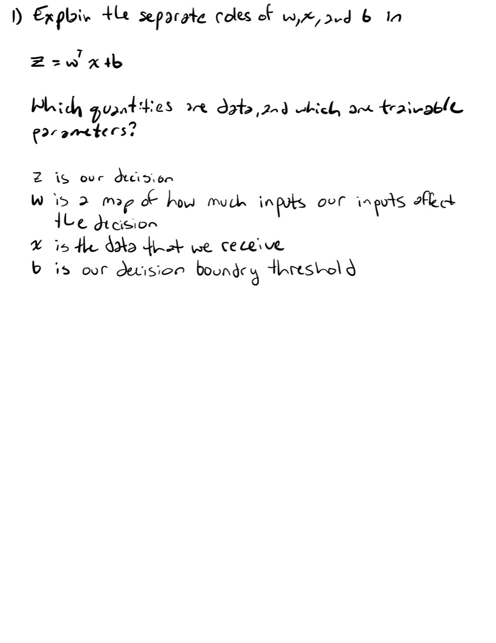
In plain language, explain the separate roles of , , and in . Which quantities are data, and which are trainable parameters?
-
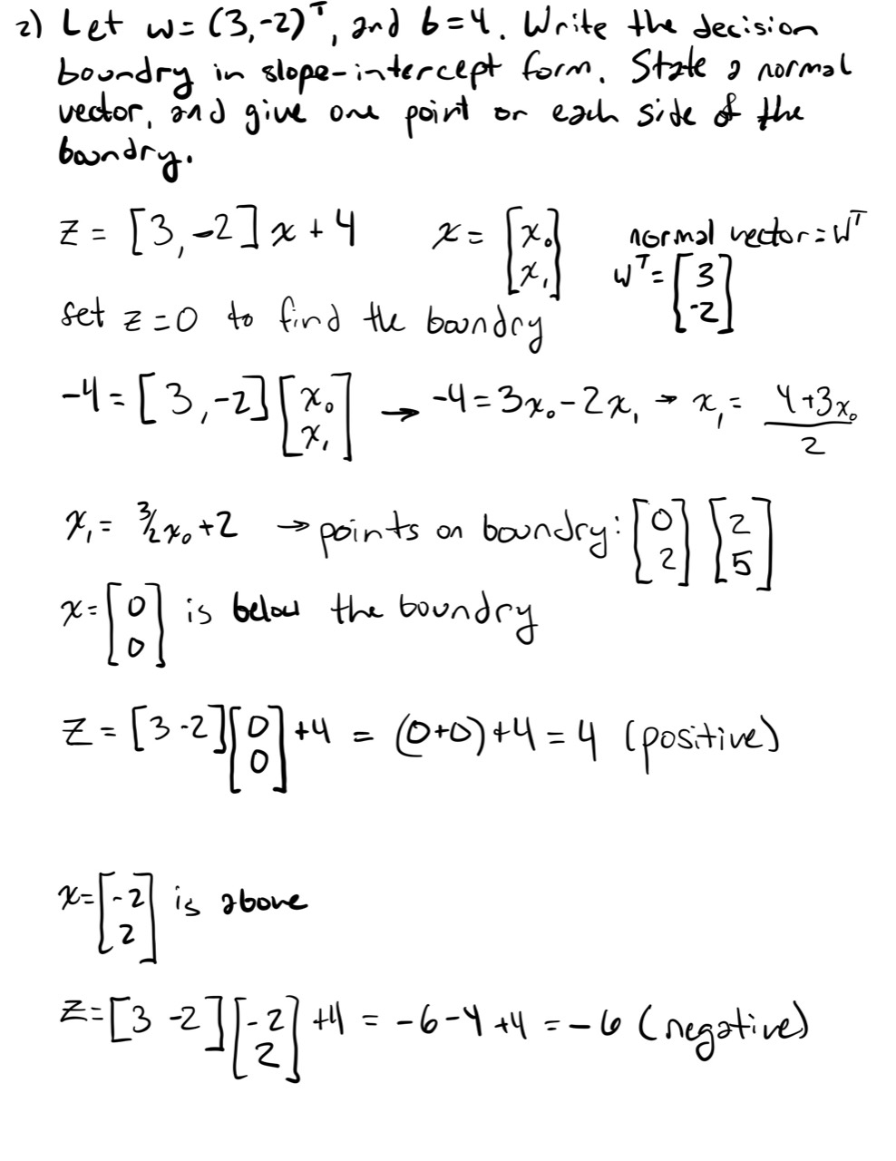
Let and . Write the decision boundary in slope-intercept form. State a normal vector and give one point on each side of the boundary.
-
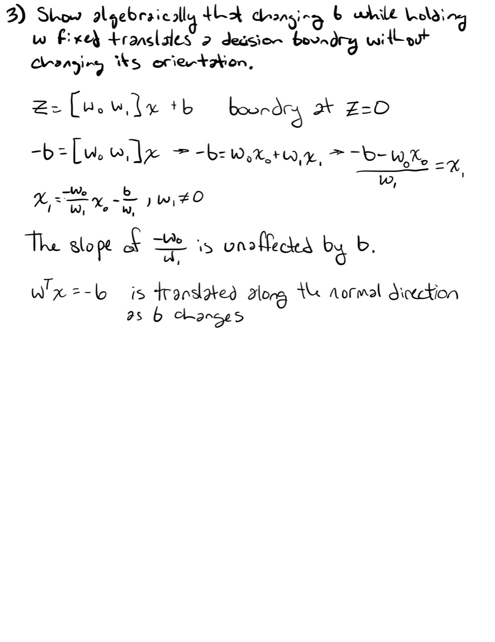
Show algebraically that changing while holding fixed translates a decision boundary without changing its orientation.
-
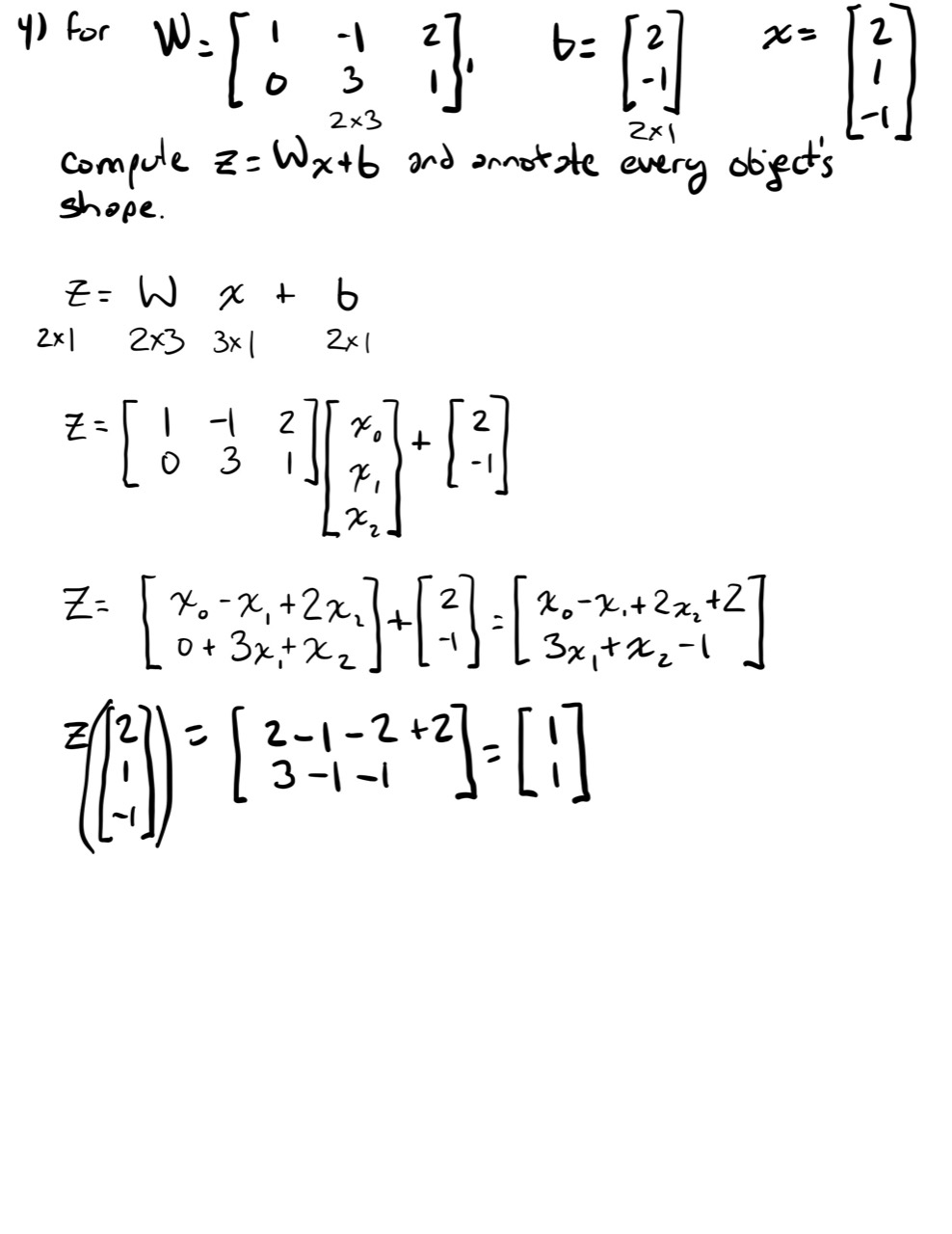
For:
compute and annotate every object’s shape.
-
Let and . Derive , , and using the chain rule.
-
Prove that two affine layers without an intervening nonlinearity can be represented by one affine layer. Identify the combined weight matrix and bias vector.
-
For , derive , , and from the differential:
Use the Frobenius inner product to identify the matrix gradient.
-
A ReLU unit receives . What output and local derivative does it produce? What practical training problem can occur if a unit remains in this region for every example?
-
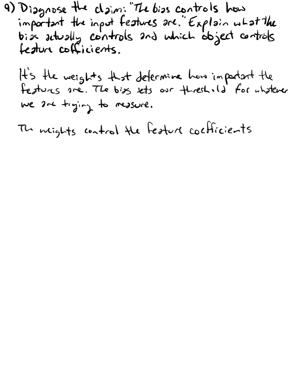
Diagnose the claim: “The bias controls how important the input features are.” Explain what the bias actually controls and which object controls feature coefficients.
-
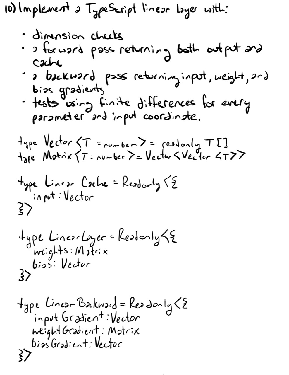
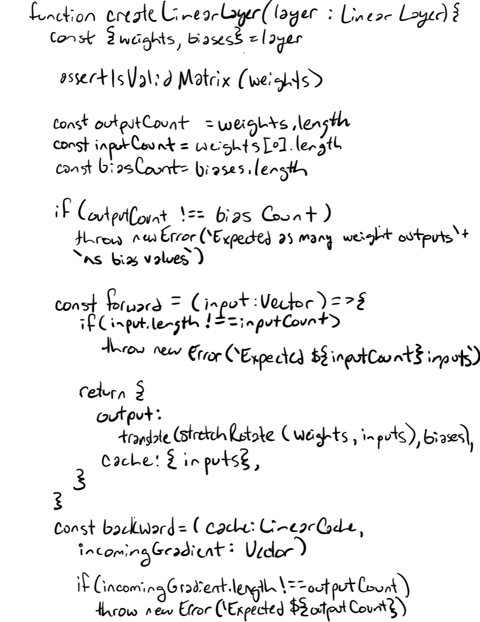
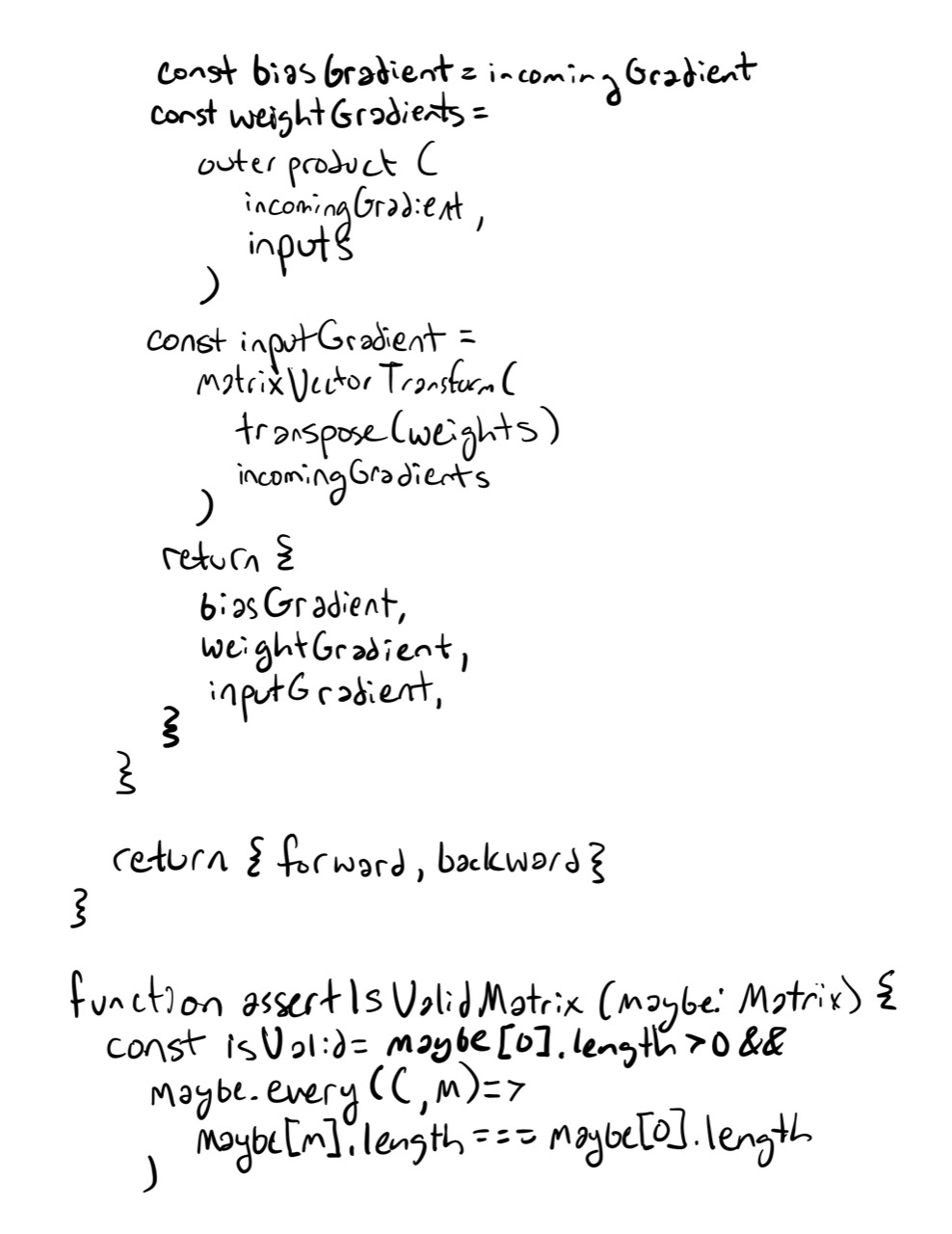
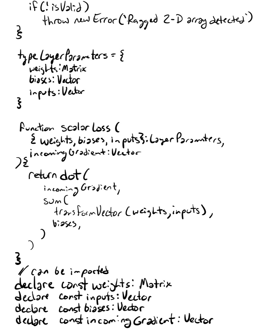
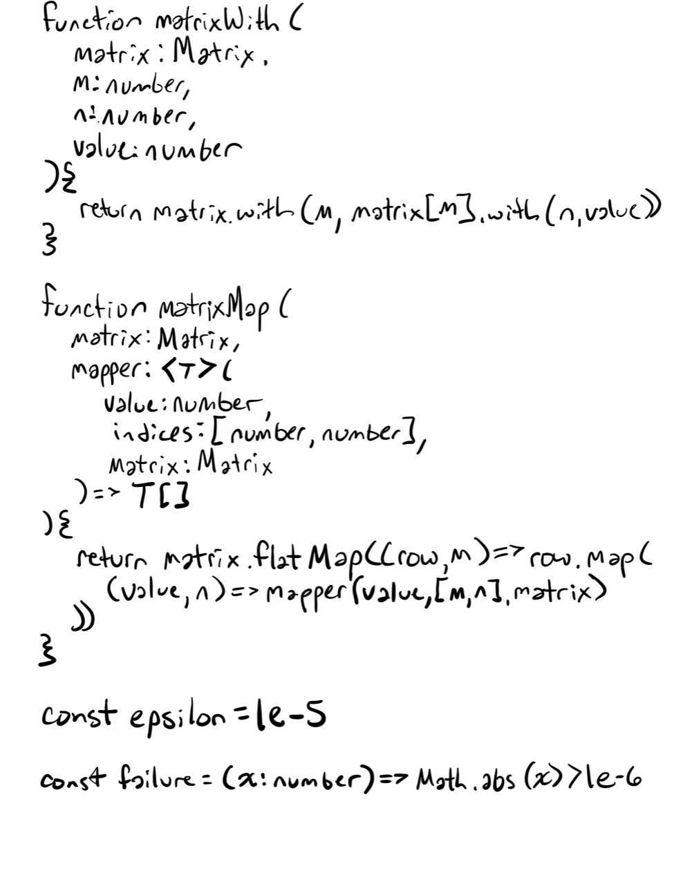
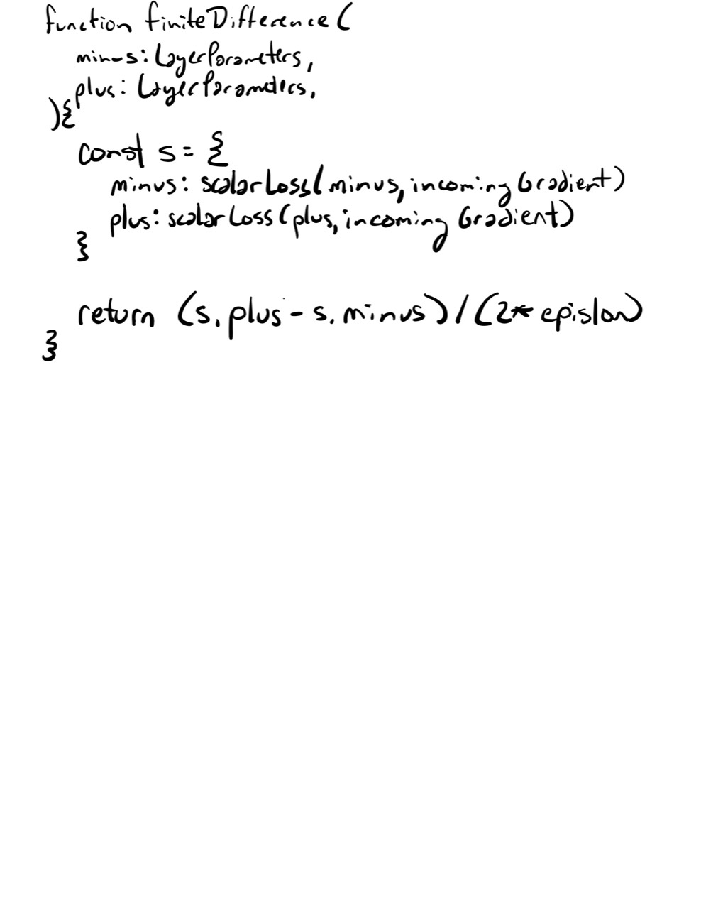
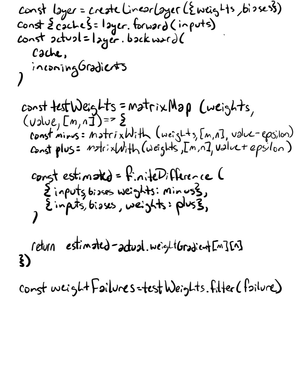
Implement a TypeScript linear layer with:
- dimension checks,
- a forward pass returning both output and cache,
- a backward pass returning input, weight, and bias gradients,
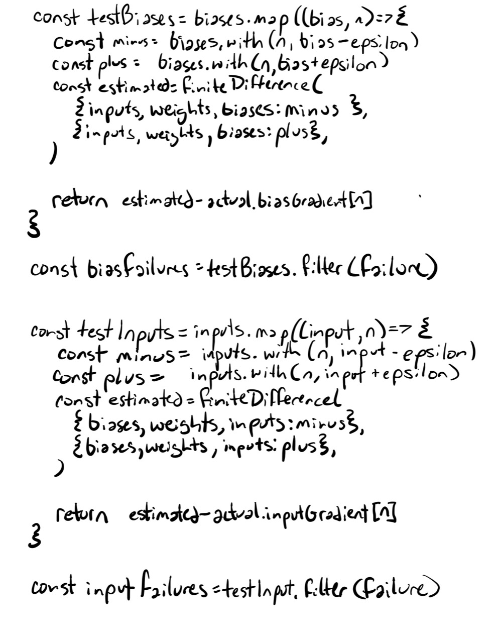
- tests using finite differences for every parameter and input coordinate.
Readiness Check
You are ready for the next lesson when you can:
- read both algebraically and geometrically,
- identify the decision boundary and its normal vector,
- generalize one unit to ,
- track every shape in the forward and backward passes,
- explain why nonlinear activations are required between layers,
- and derive the linear layer’s gradients rather than memorize them.
Summary
- A perceptron computes an affine score and applies a decision or activation rule.
- The weight vector is normal to the decision boundary; the bias translates that boundary.
- A linear layer stacks several units into .
- Several affine layers without nonlinearities collapse into one affine map.
- For a scalar loss, the linear-layer gradients are , , and .
- Linear layers are the reusable trainable maps from which larger neural networks are assembled.
Next Lesson
Lesson 41 introduces activation functions as geometric gates. It will compare sigmoid, tanh, and ReLU, study their derivatives and saturation behavior, and show how nonlinearities change the functions a network can represent.
Completed Exercises
Handwritten work submitted after completing this lesson.